The Turnantenna – Second evaluation update

Time is passing, and work is proceeding.

Last month I reported a problem concerning speed of our beloved Turnantenna: the acceleration was not constant during movement of the stepper engine, as I wanted. The error was caused by implementation of a bad algorithm. A constant acceleration is important to provide a smoother movement, and is needed to reduce the load on the engine. Force is equal to mass times the acceleration; if the acceleration is constant, so is the force; but if the acceleration grows, the stepper’s force grows as well, as long as it can keep up. Uncontrollable acceleration lead to unpredictable forces (or better, toques).

To understand the issue, a brief summary should be given: the way to control the stepper’s speed consists of changing the time between two consecutive steps. The shorter the time, the faster the movement. The previous (and wrong) algorithm, is documented in the older post. It wasn’t a good way to control a torque-limited engine because, as said before, the acceleration was not constant. In the previous algorithm, speed was taken like this:

v_n = v_n-1 + const

namely, at time tn the speed was a fixed amount more than t_n-1.
Time between two steps was

dt = (n – n-1)/v_n = 1 / v_n

It may appear correct, but the resulting graph was the following:

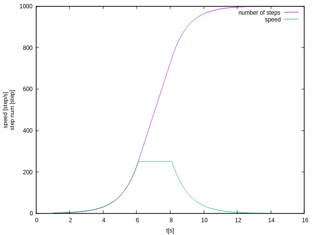
As can be seen, the speed is not linear. This mean that the acceleration is not constant, but increasing.

I found a solution thanks to a document written by Atmel Corporation. It made me think about the relationships between speed (v), space (s), time (t) and acceleration (a) that comes from physics laws:

s = a ½  t² + v₀ * t + s₀

this equation is always true, when accelerating, when the speed is constant, and even when decelerating. Quantities change inside the formula, but it always remain true.

Now, to keep it simple, let’s consider the first phase: the acceleration. A the beginning of its movement, the engine is still (v₀ = 0), and it starts without having already done one single step (s₀ = 0). The resulting equation is evaluated at v₀ =0  and s₀= 0:

s = a ½  t² + 0 * t + 0
s = a ½  t²

Now, let’s think about what is known: the acceleration a, that it is constant (because I want it so), s and t; s is the number of steps already done at time t. If I know how many steps -s- I have to do I can find how much time I have to wait –t-, and vice versa.

To find the time between two steps (the step #n and the step #n+1) the formula is:

s = a ½  t²
==>  t = sqrt(2 * s / a)

# at the step number ‘n’
t_n = sqrt(2 * n / a)

# time between step ‘n’ and ‘n+1’
dt = t_n-1 – t_n = sqrt(2 / a) * (sqrt(n+1)-sqrt(n))

Using this calculation, acceleration is constant, and speed increases linearly, as it can be seen in the graph below:

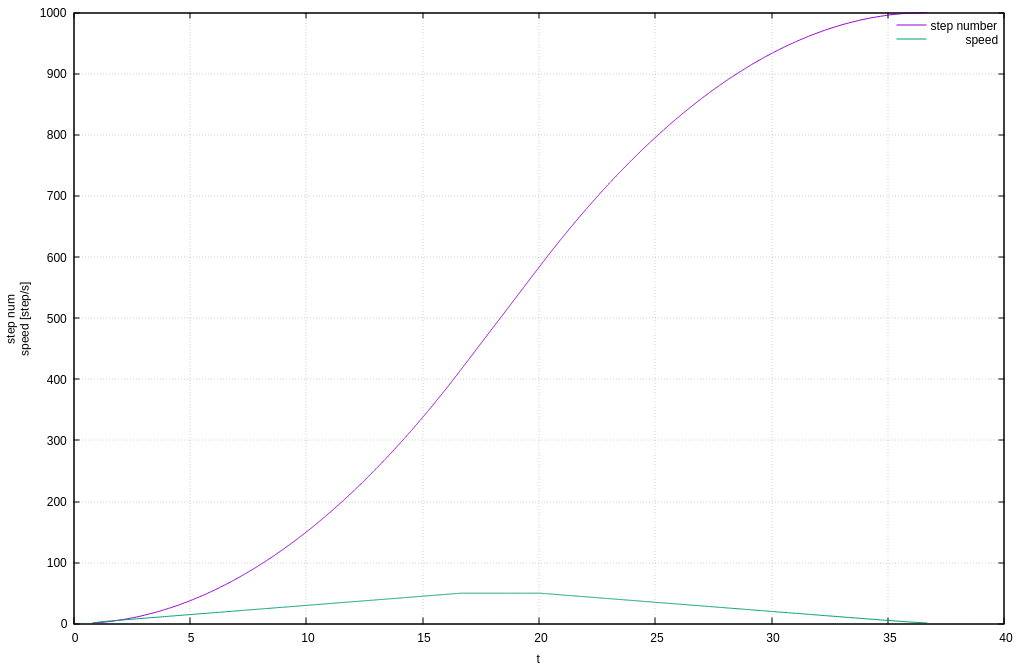
AAAAAH.. a perfect blue line! 😀

Problem: Solved!

Working on tests

Now, more progresses have been done in tests. For those who don’t knows, I’ve started my programming adventure with with this project. Everything for me is anexciting discovery, and during this month I learned and implemented the “argparse” and “logging” libraries. Now it is possible to execute the tests with three verbose levels: the first is silent, the second shows debugging informations and the third shows the info level.
It could appear trivial, but I’d never done it before, and now tests are smarter!

It is not all: I reviewed all the tests, fixed problems and improved their reliability. They’re still not perfect, but I’m working on them daily to get details right.

Fly across borders

It was time to go outside the boundaries, and to think about an interface that bring into communication the web interface and the driver. This is what I’m working on in these days.

To achieve that goal, the problem has to be studied starting from an high level. The main process, which is constantly running, float between a small number of determined states: initialising, still, moving and error handling. Together with the Ninux Florence developers community I built the following state machine graph:

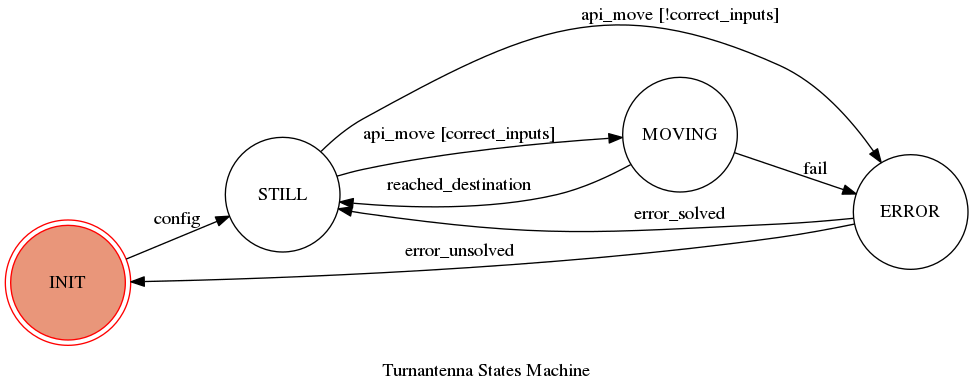
This was realized with the GraphMachine module of the “transmissions” library. Now I’m working on the full representation of this map in code lines. But there is something more.. In fact, at this point, multiprocessing became necessary to provide a safe environment: when the engine is in the MOVING state, for example, and a new command is sent to make a new different rotation, the main process should have the possibility to manage simultaneously the ongoing movement and newer requests.

That’s why we choose to keep the main process always active and make it decide when to run the movement procedure in a dedicated process, like a traffic light.

Turnantenna.me

The greatest effort, this month, was done writing down a full, detailed documentation of the project. 80 pages on what is the Turnantenna, how it works, and when and why to use it.

Many people expressed their interest in the project, someone has offered to support us but, without a complete documentation available, it is difficult to provide a starting point.

The whole doc will be soon available, and this post will be updated with the dedicated link. So, if you are interested in the project, let us know! For the moment, GitHub repository is available here.

See you next month!

— UPDATE —

The link of the full documentation of the project is provided below.
turnantenna.readthedocs.io