Hi everyone! I’m thrilled to share that I’ve successfully completed my Google Summer of Code 2025 project with Freifunk and qaul!
I’ve spent the past few months working on implementing a comprehensive RPC user authentication layer for qaul. This journey has been both challenging and incredibly rewarding, and I’m excited to share the final results of my work.
A huge thank you to my mentor MathJud for his continuous guidance and support throughout this project, and to Andibraeu and the entire Freifunk community for this amazing opportunity!
Project Overview
qaul enables peer-to-peer communication without any internet or communication infrastructure, using local wifi networks or shared phone wifi networks. My project focused on creating a robust authentication and encryption system that would lay the foundation for multi user support per node and future web interface.
Progress after mid term
Session Management System
I developed a token-based session management system. The tokens for each user are stored in their configuration file, which ensures session persistence.
Protobuf updates
Extended qaul’s RPC communication structure with new authentication modules:
This project brings significant benefits to the qaul ecosystem and its users:
For Users:
Enhanced security through proper authentication.
Ability to use multiple identities on the same node
Session persistence across application restarts
Foundation for web-based access without app installation
For Developers:
Extensible authentication framework for future features
Modular design enabling easy maintenance and updates
For the Community:
Improved scalability
Foundation for building web interfaces
Support for shared node resources in community networks
Challenges and Learning
This project presented several technical challenges that deepened my understanding:
RPC System Integration: Extending qaul’s existing RPC infrastructure required careful study of the codebase and multiple iterations to achieve integration.
Cryptographic Implementation: Implementing secure authentication without exposing passwords required the dual-hash approach with nonces, ensuring each authentication is unique.
The tradeoffs we made
We have one active session per user right now instead of multiple concurrent sessions.
We’ve tokens in the config.yaml, but we also have private keys. So, that works!
The challenge-response flow adds complexity, but ensures passwords are never shared over the network, and the whole mechanism also prevents rainbow attacks.
The known inefficiencies
Nonce is a simple counter instead of random number.
No prevension of duplicate usernames, this is the reason that causes authentication failures when multiple users share names.
Scopes of improvement
Multiple sessions per user that would enable multiple devices for a user.
Security layer for authenticated user containment in libqaul. For that a user can only execute functions it is entitled to.
Additional protobuf message to ask the system for all available users to login.
This function delivers different results, whether a user is local or a user is trying to remotely login.
Conclusion
Completing this GSoC project has been an incredible journey of growth and learning.
This isn’t goodbye 🙂 I’m excited to continue contributing to qaul and the broader freedom tech ecosystem. The future of decentralized, censorship-resistant communication is bright, and I’m honored to be part of building it!
Hello everyone! This summer as part of GSOC 2025 I’ve worked on Adding Wi-Fi Support to QEMU Simulations in Libremesh. This project consisted in “bridging” virtual machine running LibreMesh firmware using their Wi-Fi interfaces inside QEMU, in order for it to become part of the development loop of the LibreMesh.
This is my final write up for this project, and a conclusion of an enriching journey. You can also explore my first and second blogposts for Freifunk.
This project led me to learn a lot about virtualization, OpenWrt, and open source in general !
Simulating Wi-Fi within a Virtual Machine
Testing wireless communications is a tricky problem for many reasons : the medium through which the messages are being sent around being literally made out of thin air, observability is subpar and repeatability is complicated, involving hardware heavy setup.
Thankfully, mac80211_hwsim solves (most) of the issues for us. In simple terms, this module simulates Wi-Fi hardware inside the Linux Kernel, and allows us full control of it – as many Wi-Fi radios as one would want within a single machine and with complete control over it, with each of the radios able to talk to the other radios created by this module.
kmod-mac80211-hwsim
OpenWrt being based on the Linux Kernel, we should have access to this module.Even better : it’s a package ! That’s good news since now integrating this solution to our future testing will require minimal intervention : it’s a simple package to add to our build configuration.
LibreMesh virtual Wi-Fi capable firmware
So following LibreMesh instructions for building our own firmware, and by simply adding kmod-mac80211-hwsim to our configuration, we end up with exactly what we are looking for : a virtual Wi-Fi capable LibreMesh firmware.
Unfortunately, mac80211_hwsim limitless possibilities bring us some issues : LibreMesh firmware have never been tested against 6G capable router, and ends up wrongly configuring the virtual radios, preventing us from obversing the expected behaviors. This led me to dig about Wi-Fi bands and their specifications, especially 802.11ax which brings a whole set of restrictions (and confusions) especially in the upper range of the spectrum.
All in all this was beneficial to the project since I was able to provide a patch to fix the unexpected behaviors, which in the end should speed up the (future) integration of LibreMesh to 6G capable routers.
Once the fix provided, LibreMesh firmware was working as expected when run inside a QEMU virtual machine – I was able to replicate the classic AP-STA set up within the virtual machine, as is usually showcased when demonstrating the capabilities of mac80211_hwsim.
Connecting multiple virtual machines through Wi-Fi interfaces
Now that we were able to have a working virtual machine with Wi-Fi capabilities, the goal was to have multiple of these virtual machines, and to connect them to each other through their Wi-Fi interfaces, create a “virtual mesh”.
Connecting multiple QEMU virtual machines through their virtual ethernet interfaces have been a solved issue since many years (even though there is still active development in that area) due to the critical nature of the problem for the big cloud services provider, connecting multiple virtual machines through their Wi-Fi interfaces have mostly remained an afterthought, an academic project at most.
vwifi
vwifi is a project enabling simulation of Wi-Fi across multiple Linux QEMU virtual machines, relying on the mac80211_hwsim driver and finally, with specific support for OpenWrt
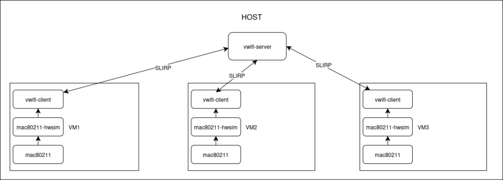
It basically relays Wi-Fi frames across the virtual machines : a server is running on the Host machine and each vms are connected to it. Inside each virtual machine, each radios are managed by the vwifi-client : each frame is passed to the server. A schematic is provided for easier understanding of the setup.
Compilation of this project for OpenWrt is a bit finicky, but manageable. A package for easier integration with OpenWrt is under development by my mentor Javier Jorge.
Virtual Mesh in LibreMesh !
Now that we have a way to create Wi-Fi frames inside a virtual machine and have it relayed to an other machine, let’s piece everything together and create our LibreMesh mesh !
Meaning that new development of features for LibreMesh such as the shared-states packages relying on heavy and cumbersome infrastructure to test and iterate will be possible by simply cloning this set of scripts inside your OpenWrt build directory, and simply running them will provide a lightweight, reliable and quick to set up testbed.
Automation of testing in LibreMesh
Last piece of this puzzle is the automation of the testing in LibreMesh.
So far, testing in LibreMesh was provided by unit testing using a docker image and mockups of the expected behavior, and manual testing using real hardware. QEMU only occured during development and wasn’t fully integrated in the development process, since it was easier and more reliable to just upload the firmware to an adjacent router and observe the behavior. But now that we proved that it was possible to set up true and reliable Wi-Fi mesh network, the next obvious step is to provide automated testing and completely integrate it in the LibreMesh development loop.
OpenWrt-test
OpenWrt-test is a labgrid test based framework aiming at providing worldwide testing for OpenWrt across multiple devices. I’ve had the opportunity to meet up with the main developer of this project apacar during BattleMeshv17 and with my mentor and the LibreMesh community we decided to based our future QEMU based testing on this framework, since it is tightly integrated with OpenWrt and also based on the convenience when wanting to run the tests across different devices.
To use it, OpenWrt-test have to be cloned inside the OpenWrt build directory, and then a Makefile will handle the rest of the setup.
make tests/qemu-x86-64 V=s will allow you to run the different tests (specific to OpenWrt) located inside the tests/ directory of the project.
The project have been forked in order to provide specific test to LibreMesh : despite being based on OpenWrt, LibreMesh still show some specific differences. And finally, after a lot of struggle, I was finally able to integrate LibreMesh inside this framework with the rest of my work.
The setup consists in :
starting the virtual LibreMesh mesh and setting up each of the VM,
Running the labgrid test
Labgrid will then spin up its own virtual machine based on the latest build present in bin/target/x86/64 and then be able to connect to the virtual Wi-Fi mesh, and run automated test against the infrastructure. This allows to run repeatable tests in a controlled manner, orchestrate 4 different machines and quickly iterate when developing new feature requiring some specific Wi-Fi setup.
Future Work
This project managed to showcase the repeatability and convenience of Labgrid for automated tested, which coupled with the ability to create virtual Wi-Fi meshes brings a whole new worlds of possibilities for LibreMesh development, as well as any Wi-Fi mesh features : lightweight infrastructure, quick setup and fully repeatable.
Future work will concentrate on bringing better coverage for LibreMesh testing using the new tools that are now proven to be effective from this GSOC project. So far testing covers part of the shared-state packages, but different packages could be targeted, and not only the ones relying on a Wi-Fi mesh network but also general configurations.
Lastly, vwifi document way to introduce packet loss as well as nodes mobility : this could allow for different scenario of testing and bring a whole new set of robutness to the LibreMesh project.
Conclusion
This Google Summer of Code provided me the opportunity to discover many new things : I broaden my understanding of Wi-Fi and even discovered new use cases for it, tinkered with it in the Linux Kernel, learned about OpenWrt and LibreMesh and more importantly met with incredible and very passionate people.
I’m very thankful to have been able to work on such a project during this summer, and would like to thank very fondly my mentor Javier Jorge for his support throughout this adventure.
Thank you also to Freifunk for allowing this to happen, it’s really a fantastic opportunity for everyone involved.
I will definitely continue to contribute to LibreMesh and OpenWrt and hope to meet with you in person at BattleMeshv18!
Hi everyone! Welcome back to the final blog post in this series on Deep Q Network-based Rate Adaptationfor IEEE 802.11ac Networks. The goal of this project is to build an intelligent rate control mechanism that can dynamically adapt transmission rates in Wi-Fi networks using Deep Reinforcement Learning.
Modern Wi-Fi networks need to dynamically pick a suitable Modulation and Coding Scheme (MCS) index based on ever-changing channel conditions. Choosing a rate that is too high relative to the channel quality (e.g., under high attenuation of interference) in a noisy channel typically leads to packet losses, while selecting a very conservative, low rate wastes valuable airtime, which ultimately harms the user experience. Traditional rate adaptation algorithms such as Minstrel rely on heuristics and fixed averaging windows, which may not generalize well across different environments or capture complex temporal relationships between link-layer feedback and optimal rate decisions. In this GSoC project, we explored a Deep Reinforcement Learning (DRL) approach to rate adaptation for IEEE 802.11ac networks. Specifically, we implemented a Deep Q-Network (DQN)-based algorithm that learns to select optimal data rates directly from real-world observations derived from the ORCA (Open-source Resource Control API) testbed. We aimed to develop an intelligent controller capable of maximising throughput while maintaining a high transmission success ratio, without relying on handcrafted rules.
This blog walks through our journey: how we built an offline Wi-Fi rate adaptation environment from scratch, how we trained a DQN agent using real-collected packet-level traces, what technical challenges we faced along the way, and how the learned policy compares to traditional approaches.
Please feel free to check out the introductory and the mid-term blogs for more background details.
2. ORCA and Rateman [1]
To carry out this project, we leveraged ORCA, a kernel-user space API that exposes low-level transmission statistics and allows runtime control over Wi-Fi parameters including Modulation and Coding Scheme(MCS) index, defined by modulation type, coding rate, bandwidth, guard interval, and number of spatial streams. It enables remote monitoring and control from user space using the Remote Control and Telemetry Daemon(RCD). RCD is a user space package connecting ORCA endpoints to a bidirectional TCP socket, forwarding monitoring data and control commands.
ORCA allowed us to configure Access Points (APs), Stations (STAs), and capture real-time feedback such as Received Signal Strength Indicator (RSSI), frame attempt and success counts, and estimated throughput.
On top of ORCA, we utilize RateMan, a Python-based interface that simplifies per-STA rate adaptation and integrates cleanly with real-time experimental setups across multiple APs. It provides a clean abstraction to implement custom resource control algorithms in the user space.
This tight ORCA–RateMan integration allowed us to record realistic wireless behaviour under varying conditions, and later replay those traces in a simulated RL environment, effectively combining the benefits of real-world data with the repeatability and efficiency of offline learning.
Fig 1. Overview of the architecture of the user-space resource control using RateMan via ORCA [1]
3. Project Goals
The main goal of this project was to investigate the viability of Deep Reinforcement Learning for Wi-Fi rate adaptation and to build an end-to-end system capable of learning from real-world wireless behavior and deploying intelligent rate decisions on commodity hardware. To achieve this, we defined the following concrete objectives:
Design a custom offline training environment tailored to Wi-Fi rate adaptation, where step-wise interaction is simulated using real packet-level traces instead of synthetic models.
Leverage passively collected data where a fixed MCS rate is used throughout ORCA experiments. These traces — containing attenuation levels, RSSI values, success ratios, and throughput — serve as the experience source for training the DQN agent.
Implement a Deep Q-Network (DQN) learning pipeline in PyTorch, chosen for its flexibility, fine-grained control over training primitives, and compatibility with Python 3.11 (required by ORCA-RateMan setup). Our implementation includes all major RL components, replay memory, epsilon-greedy agent, target network, and Bellman update, customized to our environment and thus can be considered a “from-scratch” integration, rather than relying on high-level RL libraries.
Develop a DQN-based rate adaptation logic that plugs into RateMan’s user-space API, enabling learned actions (rate indices) to be sent to the real Wi-Fi firmware in a closed-loop fashion.
Benchmark the learned agent against classical heuristics, with Minstrel-HT chosen as the baseline due to its widespread use in Linux Wi-Fi stacks.
Ensure full compatibility with ORCA testbed hardware, so that the trained model and logic can be transitioned from offline simulation to real deployments without modifying the low-level radio stack.
These goals collectively shaped the backbone of our GSoC journey, from data collection and environment design, through learning and experimentation, to hardware-ready integration.
4. DQN Basics
A Deep Q-Network (DQN) is a reinforcement learning (RL) algorithm that uses deep learning to estimate the Q-function, which represents the cumulative reward of taking an action in a given state.
Fig 2. Illustration of state, action, and reward sequence in the interactions between the agent and environment within the reinforcement learning algorithm [4]
Environment Design
State Representation: [rate, attenuation, RSSI, success_ratio] : In our offline training setup, each state is represented by a four-dimensional vector consisting of the transmission rate, attenuation, RSSI, and success ratio. The rate corresponds to the MCS index, which is directly obtained from the logged transmission events and defines the PHY data rate attempted by the access point. The attenuation reflects controlled channel conditions that were introduced during the experiments using programmable attenuators, thereby simulating realistic wireless environments with varying link degradation in decibels. The RSSI (Received Signal Strength Indicator) is extracted from the receiver-side logs and provides a direct measure of the signal quality experienced by the station, serving as an important feature that correlates link quality with achievable throughput. Finally, the success ratio is computed from ORCA’s transmission counters as the fraction of successful transmissions over total attempts within a logging interval, capturing the reliability of the chosen rate under the given conditions. By combining these four parameters, the state representation captures both the controlled experimental setup and the resulting link quality, offering the reinforcement learning agent the necessary context to make informed rate adaptation decisions.
Action Space: Initially considered all valid 802.11ac rates, later narrowed down based on practical feasibility and dataset coverage.
Reward Function: Directly proportional to achieved throughput, while penalizing low success ratios (to discourage risky selections).
Agent and Learning Logic
The agent uses ϵ-greedy as the exploration strategy that selects random actions with probability ϵ, otherwise selects the action with the highest predicted Q-value.
Replay Buffer: Stores past experiences to break temporal correlations during training.
Q-Network: A neural network parameterized with weights, mapping states to Q-values for every possible action.
Target Network: A periodically updated copy of the Q-network to stabilize learning.
The agent iteratively samples experiences from the replay buffer and minimizes the Bellman loss, learning to associate long-term throughput gains with specific rate decisions under varying channel conditions.
Hyperparameters
The following hyperparameters were used during training:
Discount factor (γ = 0.99): Balances immediate vs. future rewards. A high γ ensures the agent values long-term throughput instead of being greedy about short-term gains.
Batch size (128): Number of experiences sampled from the replay buffer for each training step. Larger batches provide more stable gradient updates.
Learning rate (1e-3): Controls the step size in updating network weights. A moderate learning rate ensures steady convergence without overshooting.
Target update frequency (1000 steps): Determines how often the target network is updated with the Q-network’s weights. This reduces instability during training.
These hyperparameters ensure that the agent can generalize effectively from past experiences, avoid instability in Q-value estimation, and steadily converge toward optimal rate adaptation behavior.
5. Setup
For data collection, all experiments were conducted using two RF isolation boxes, one housing the ORCA-controlled Access Point (AP) and the other housing the Station (STA). The antenna ports of the AP and STA were connected via RF cables, with an Adaura AD-USB4AR36G95 4-channel programmable attenuator placed in between. Figure 1 provides a visual illustration of the setup.
This enclosure ensures a controlled wireless environment free from external interference, noise, and multipath effects. This allowed us to precisely evaluate how different MCS rates behave purely under varying attenuation levels.
Using programmable RF attenuators inside the box, we could emulate varying channel qualities in a deterministic way, while keeping other environmental variables fixed. This level of controllability is vital when generating training data for RL agents, as it guarantees that observed effects in performance are attributable primarily to rate selection and attenuation.
5.1 Data Collection
Hardware/Testbed: ORCA nodes with RateMan control loop.
Configuration: AP ↔ STA, static distance, attenuation swept gradually.
Rates Tested: One rate group per experiment — e.g., Group 12 (120-128(hex) ⇒ decimal 288–296). Each group contains indices for different modulation type and coding rate, for fixed number of spatial streams, bandwidth, and guard interval. (more details in the mid-term blog)
Parameters Extracted (from raw trace files): rate, attenuation (dB), RSSI (dBm), theoretical_data_rate (Mbps), and number of attempted and successful transmissions.
Calculated Features:
success_ratio = successful / attempted
Used to compute state vectors and rewards for the offline RL environment.
5.2 Reward Function Variants Tested
Designing the reward was critical, as it directly influenced which rates the agent learned to prefer:
reward = success_ratio × throughput
Simple and intuitive, but failed to penalize high rates that recorded zero successes. These rates often had theoretical throughput, misleading the agent into over-selecting them.
Integrated punishment for unreliability, but was too harsh on high rates, causing the agent to ignore them even under good channel conditions.
Attenuation-aware penalty
Penalizes failed transmissions, scaled by attenuation, so the agent learns to accept occasional failures at low attenuation (where high rates are viable), but becomes conservative at high attenuation, where such attempts are wasteful.
All generated experience tuples were stored in .pkl files, one per rate group experiment. These served as the replayable dataset for our offline DQN training pipeline.
5.3 Environment Design
Offline Training Environment To train our DQN agent, we constructed a simulated environment that replays experiences extracted from the .pkl trace files collected on the ORCA testbed. At each time step, the environment provides the state representation [rate, attenuation, RSSI, success_probability], exposes the available rate indices from the corresponding group as the action space, and computes the reward using the designed function described in Section 5.1.
Training proceeds entirely offline: the agent never interacts with real hardware during this stage. Instead, the training loop samples batches of transitions from a replay buffer, computes the Bellman loss, and iteratively updates the Q-network weights. This approach allowed us to leverage large amounts of pre-recorded data efficiently while avoiding the practical limitations of online learning.
Post-Training Simulation Environment After training, the learned DQN models were evaluated in a separate simulation environment designed to mimic—but not directly replay—the collected traces. Unlike the training phase, the evaluation relies solely on the learned Q-function. Given the current attenuation level, the DQN selects an action (rate index), and the simulator generates the corresponding success probability and reward using the theoretical data rate of that action to approximate real-world performance.
This evaluation loop enabled us to benchmark the generalization ability of the DQN policy, independent of the training samples, and to assess its rate-selection behavior under different attenuation conditions before attempting live deployment.
5.4 Deployment via Rateman (Live Testing Environment)
Once satisfactory results were obtained in simulation, the trained DQN policy was deployed inside the RF shielding box, where the real wireless medium served as the environment. In this setup, RateMan acted as the control and monitoring interface to ORCA. At each decision interval, RateMan queried the Python-based DQN model for the next rate index, pushed the chosen rate to the ORCA firmware, and collected live link-layer statistics such as attempted transmissions, successful packets, and RSSI. These statistics were then fed back to the DQN logic for subsequent decisions.
This creates a closed control loop: DQN policy → RateMan control API → ORCA hardware → real radio environment → feedback to DQN.
Fig 3. Current DQN Implementation
5.5 Model Evaluation
Following the successful integration of the trained DQN with the RateMan control loop, we wanted to test the efficiency of the trained DQN model on a simulated environment that mirrored the real wireless testing setup.
To visually inspect whether the agent was making sensible decisions, we generated heatmaps showing which rates were chosen across different attenuation values, revealing if the DQN correctly preferred higher rates at lower attenuation and more conservative rates as channel quality degraded.
Fig 4. Rate-Attenuation(55dB) Heatmap
Figure 4 illustrates a heatmap indicating how each of the 232 available rates behaves at that attenuation. The success ratio is indicated by the background color of each cell, with purple and red being the extreme positive and null successes. Each cell also contains its theoretical data rate, upon which our reward system is based. So, in this case, we would expect the DQN model to select the rate (4,80Mhz, 400ns), (16-QAM,¾) as its theoretical rate is the highest among the successful rates.
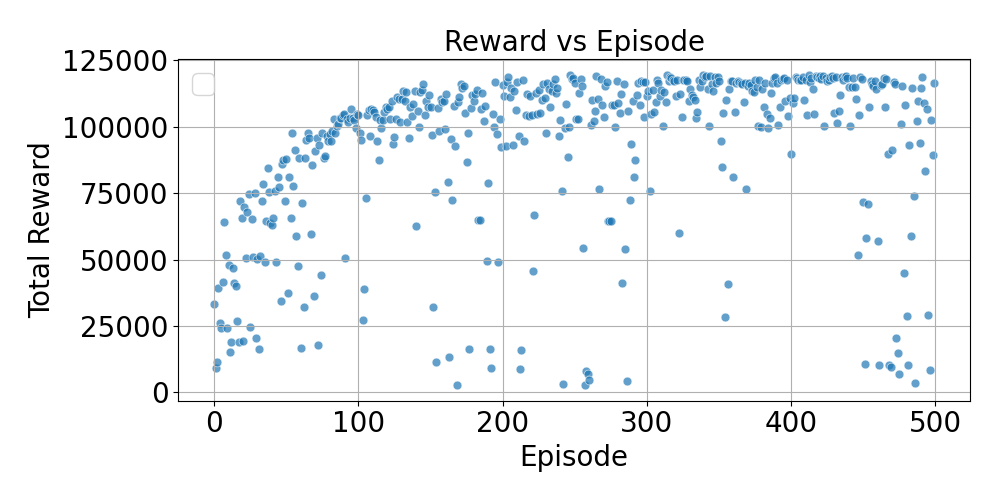
We then plotted reward curves over multiple episodes to assess overall stability and performance. Figure 5 expresses the efficiency of the trained DQN model to generate ample rewards (based on theoretical data rates) throughout the entire period.
Fig 5. Distribution of rewards over time
After the confirmation of positive rewards, we conducted live experiments in the shielding box to evaluate the real-world behaviour of the learned rate adaptation policy.
For each run, we swept attenuation levels and continuously logged:
Rate index selected by the (Deep Q-Network based Rate Adaptation) DQN-RA
Expected throughput, success probability, and reward
Corresponding attenuation (dB) and RSSI
Then we benchmarked the distribution of selected rates against manually known “optimal” rates for different attenuation regions using the above-described heatmaps.
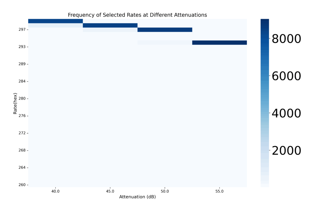
Fig 6. Selected Rates at different attenuations
In Figure 6, we can observe the frequency of different rates selected at each attenuation. With the help of the heatmaps described above, it was confirmed that the DQN model was indeed selecting the highest feasible rates and thus maximizing its rewards.These analyses helped verify that the DQN was not only compatible with RateMan in deployment, but was also making reward-maximising, context-aware decisions in a live RF environment.
Results
The performance of the deployed DQN agent was assessed by analysing its rate-selection behaviour under varying attenuation levels compared to minstrel_ht.
We ran experiments with minstrel_ht and DQN-Rate-Adaptation under similar settings.
For the DQN, scatter plots and heatmaps revealed clear switching behaviour with higher MCS rates chosen at low attenuation (strong channel conditions), and lower, safer rates selected as attenuation increased.
Figures below summarize the comparison against minstrel_ht.
Fig 7. Rate Selection for Minstrel_HT vs. DQN_RA
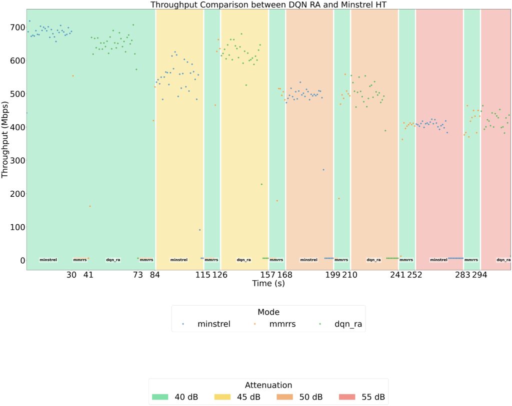
Fig 8. Measured Throughput for Minstrel_HT vs. DQN_RA
Key Observations Our experiments revealed several important insights into the behavior of the DQN-based rate adaptation algorithm. First, the learned policy adapts intelligently to changing channel conditions, consistently producing more robust rate decisions than Minstrel_ht, particularly in the mid-attenuation region where Minstrel tends to select much lower rates. This highlights the ability of the DQN agent to capture patterns in the environment that a heuristic-based approach may overlook.
When comparing throughput performance, both DQN-RA and Minstrel_ht achieve similar results at 40 dB attenuation for the same rate selections. However, as attenuation increases, DQN-RA consistently outperforms Minstrel_ht, achieving noticeable throughput gains at higher link attenuation levels. This suggests that reinforcement learning can provide tangible benefits in more challenging channel conditions.
Another interesting observation is that the agent does not simply converge to the highest theoretical MCS indices. Instead, certain rates were consistently favored because they offered stable real-world performance across a broader operating range. This indicates that the DQN agent is learning meaningful, deployment-relevant strategies rather than just overfitting to peak values.
Finally, the experiments demonstrated the importance of action space design. When the agent was allowed to explore the full set of supported rates, the learning process became significantly harder, leading to slower convergence and repeated suboptimal choices. In contrast, reducing the action space to task-specific subsets improved both practicality and performance, suggesting that action-space reduction is a critical consideration for real-world deployments of learning-based rate adaptation.
7. Challenges Faced
Throughout the development and deployment of the DQN-based rate adaptation system, several practical and algorithmic challenges emerged:
Choosing an Appropriate Training Strategy Designing an effective learning pipeline required striking a balance between offline replay-based training (easy to scale but limited by logged data) and online interaction (more realistic but time-consuming and hardware-dependent). Selecting the right blend was critical to ensure real-world deployability without overfitting to historic traces.
Impact of Action-Space Size We observed that the size of the rate action set had a significant impact on learning stability. Training with a larger action space caused Q-values to be noisy and slowed convergence, whereas a reduced, experiment-specific set led to faster and more consistent learning.
Comparison Runs (Large vs Small Action Space) Side-by-side offline training runs confirmed that smaller action spaces enabled the agent to focus on realistic rate assignments, whereas larger action sets often caused it to explore impractical high-MCS actions that performed poorly in practice.
Dangerous High-Rate Actions Certain MCS indices provided very high theoretical throughput, which yielded high Q-values early in training. But these rates were actually rarely successful under higher attenuation, misleading the agent unless penalised correctly.
Reward Shaping Difficulties Extensive experimentation was required to design a reward function that rewarded aggressive, high-performing rates under good conditions, while heavily penalising them under poor channel conditions. Several hand-crafted reward structures were tested before arriving at a formulation that maintained a healthy spread of Q-values across the action-space and prevented domination by overly optimistic, unreliable rate choices.
These insights highlight the importance of domain-aware RL design, where subtle choices in environment, rewards, and action spaces dramatically influence real-world behaviour.
8. Limitations
While the project successfully demonstrated the feasibility of DQN-based rate adaptation, several limitations were observed:
Large Action Space Challenge
Training with all 232 supported 802.11ac rates caused unstable learning and poor convergence
Restricted Evaluation Range
Experiments were limited to four attenuation levels (40, 45, 50, 55 dB), which may not fully capture the dynamics of real-world wireless environments.
Hyperparameter Sensitivity
Training stability was found to be sensitive to hyperparameter choices, highlighting the need for systematic hyperparameter tuning.
Offline Trace Dependence
The agent relied heavily on pre-collected traces, which may limit adaptability to unseen channel variations during deployment.
9. Future Work
Moving forward beyond GSoC, our objective is to progressively expand both the dataset and action space, ultimately scaling back up toward full-rate adaptation across all supported MCS indices.
Looking ahead, there are several promising directions for future work. More diverse traces can be gathered across wider attenuation ranges and channel conditions to improve generalization. Another approach can be online learning, allowing the agent to continuously adapt to real-time conditions rather than being confined to pre-collected data. Finally we can also explore advanced architecture such as Multi-headed DQNs to handle the large number of action spaces and hopefully enhance stability and performance.
This staged strategy will help maintain training stability while inching closer to a fully generalizable DQN-driven rate control mechanism for Wi-Fi systems.
10. Conclusion
The project achieved its goal of developing and deploying a DQN-based rate adaptation policy on commodity Wi-Fi hardware. By reducing the action space to a manageable subset, the agent was able to learn context-aware policies that aligned with real-world performance expectations.
Importantly, this work advances beyond earlier DRL-based rate control proposals such as DARA [2] and SmartLA [3], which focused on limited subsets of rates (often <10 actions), small variations in RSSI, and did not perform live hardware deployment on ORCA-like setups. In contrast, our system trains on genuine 802.11ac traces, integrates seamlessly with RateMan, and is fully deployable on real hardware, achieving live closed-loop decision making.
I am deeply grateful to have had the opportunity to be a part of this GSoC project. This experience has been both challenging and immensely rewarding, allowing me to explore the intersection of deep reinforcement learning and wireless networking in a real-world setting.
I would like to sincerely thank my mentors for their invaluable guidance, patience, and support throughout the journey. Their insights and encouragement have been crucial in navigating both technical challenges and research decisions.
Working on this project has been a truly enjoyable experience, and I am thankful for the chance to contribute to advancing intelligent Wi-Fi rate adaptation. This opportunity has not only expanded my technical skills but also deepened my appreciation for collaborative, cutting-edge research.
References
1. Pawar, S. P., Thapa, P. D., Jelonek, J., Le, M., Kappen, A., Hainke, N., Huehn, T., Schulz-Zander, J., Wissing, H., & Fietkau, F.
Open-source Resource Control API for real IEEE 802.11 Networks.
2. Queirós, R., Almeida, E. N., Fontes, H., Ruela, J., & Campos, R. (2021).
Wi-Fi Rate Adaptation using a Simple Deep Reinforcement Learning Approach. IEEE Access.
3. Karmakar, R., Chattopadhyay, S., & Chakraborty, S. (2022).
SmartLA: Reinforcement Learning-based Link Adaptation for High Throughput Wireless Access Networks. Computer Networks.
This summer I focused on removing LibreMesh-specific glue where OpenWrt already has a solid upstream solution, and on tightening integration with OpenWrt services:
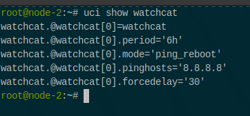
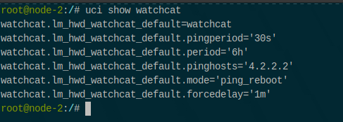
Task 1 — Reboots via OpenWrt’s watchcat: new lime-hwd-watchcat module generates /etc/config/watchcat from LibreMesh UCI and reloads the service automatically. It replaces the custom deferrable-reboot.
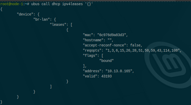
Task 2 — Move DHCP to odhcpd + cluster-wide lease sharing: prototype package that makes odhcpd the main DHCPv4 server (maindhcp=1) and shares leases across nodes via CRDTs, using ubus and leasetrigger.
Task 3 — Remove VLAN wrappers from Babel: PR switches lime-proto-babeld to run on base ifaces and br-lan (DSA), adds a small nftables guard to avoid L2 multicast leaking Babel traffic from bat0 into the bridge.
Task 4 — Plan for an L3-only LibreMesh profile: opened an L3-only mesh issue (no batman-adv/anygw) to scope the work and collect feedback.
Project goals
Simplify LibreMesh by adopting OpenWrt-native components when they are equivalent or better.
Reduce maintenance burden in LibreMesh packages by deleting code where upstream covers it.
Keep behavior observable & testable with CI/unit tests and simple field tests on real routers.
What was built
1) Integrate OpenWrt’s watchcat via LibreMesh HWD
Why: OpenWrt ships watchcat for scheduled reboots/network checks. Using it upstream avoids reboot logic and gains a familiar UI.
What: lime-hwd-watchcat (Lua) reads LibreMesh UCI (config hwd_watchcat), generates the corresponding /etc/config/watchcat sections, cleans stale ones, and reloads the service. The package lives in lime-packages and targets stock OpenWrt watchcat.
Result: Reboots and connectivity checks are handled by upstream watchcat, visible in LuCI, with configuration owned by LibreMesh.
2) Replace dnsmasq DHCP with odhcpd
Why: odhcpd is OpenWrt’s native DHCP/RA daemon, well-integrated with ubus, and already authoritative for IPv6; enabling it for IPv4 simplifies the stack.
UCI defaults set dhcp.odhcpd.maindhcp=1, point leasetrigger to our publisher, and register a community scoped CRDT.
Publisher: on lease change, call ubus dhcp ipv4leases, distill to IP → {mac, hostname}, publish to CRDT.
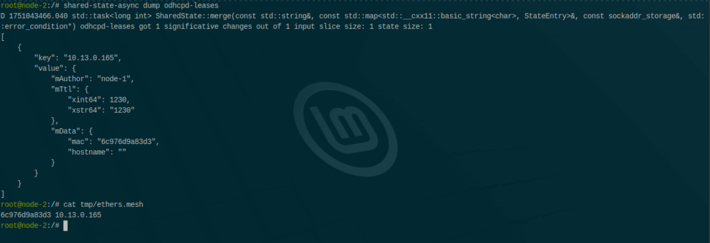
Generator: on CRDT updates, atomically write /tmp/ethers.mesh and reload odhcpd so foreign leases are served locally too. (“Leasetrigger” behavior is an odhcpd feature used here to emit on lease changes.)
In the field: two LibreMesh nodes converge on the same lease table within seconds; uci show dhcp reflects maindhcp=1. Tech references for odhcpd and UCI options: docs & source.
3) Remove VLAN interfaces from Babel (run on base ifaces / br-lan)
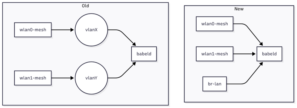
Why: Historically LibreMesh created per-radio VLANs for Babel. On modern DSA targets this adds complexity and hides interface intent. Running babeld on br-lan (wired) and radios directly is simpler and yields the right link metrics by default.
What: rewrites lime-proto-babeld to:
Configure Babel on base ifaces and add a br-lan interface (type=wired).
Drop the legacy “VLAN-on-wlan” indirection.
Add a small nftables ingress guard on bat0 to prevent Babel L2 multicast flooding into br-lan, which could otherwise create “ghost wired neighbors”. (Babel uses UDP 6696 and link-local multicast ff02::1:6 / 224.0.0.111; the guard drops those on bat0.)
Notes: The PR targets DSA (not swconfig). It also documents what to add in lime-node to enable babeld proto explicitly. See PR conversation, examples and nftables snippet.
What: Today LibreMesh typically mixes BATMAN-adv (L2) and Babel (L3): BATMAN-adv makes the whole mesh look like one big Ethernet (single broadcast domain), while Babel does hop-by-hop IP routing. An L3-only profile would switch fully to Babel for mesh connectivity, drop BATMAN-adv and anygw, and give each node its own LAN prefix.
I opened an issue to scope the work: goals, migration path, and checks the community can run while we iterate.
Before (BATMAN-adv + anygw): clients across the mesh often see the same IPv4 gateway address; the mesh feels like one flat LAN.
After (L3-only): each node runs a DHCP server for its /24 (or /64 in IPv6). Clients connected to node A live in A’s subnet; traffic to node B’s subnet routes via Babel.
Drop L2 mesh: exclude BATMAN-adv bits (lime-proto-batadv, ubus-lime-batman-adv) and remove anygw.
Keep it pure L3: enable Babel (lime-proto-babeld) on mesh radios and on br-lan. (Related: my PR removes the legacy VLAN-on-wlan layer so Babel runs directly on the base ifaces.)
Per-node addressing: use LibreMesh’s main_ipv4_address/main_ipv6_address patterns to give every router its own LAN prefix.
DHCP/RA: ensure a DHCP/RA server per node.
Gateways: if you want “plug Internet anywhere,” pair L3-only with babeld-auto-gw-mode so default routes are advertised only when WAN is healthy.
Current state (as of Aug 25, 2025)
watchcat integration: packaged in lime-packages (app + docs page) and usable today; config lives in LibreMesh UCI, rendering to standard OpenWrt watchcat.
odhcpd migration: working prototype with CRDT lease sharing; evaluation and broader testing tracked in Issue #1199.
Babel changes:PR #1210 open with review/approvals from maintainers.
L3-only profile:Issue #1211 open for community discussion and follow-ups.
What’s left / next steps
watchcat: collect feedback from communities and tune sane defaults per device profiles.
odhcpd: expand tests (IPv6 RA/DHCPv6 + v4 coexistence), harden failure modes, and benchmark lease propagation on dense meshes. Track in #1199.
Babel PR #1210: finalize DSA docs, test swconfig fallback or explicitly gate to DSA-only in code, and validate the bat0 ingress guard on more topologies.
L3-only: produce a minimal profile, migration guide (no batman-adv, no anygw).
Lessons learned
Upstream keeps projects healthy. Using existing, maintained components cuts long-term maintenance and aligns you with a larger ecosystem.
Small, reviewable changes earn fast feedback. I saw how clear PR descriptions, minimal diffs, and reproducible test notes make reviews smoother, because maintainers can reason about the change quickly.
Communication is part of the code. Good issues/PRs explain why, not just what; they show logs, decisions, and trade offs.
Deleting code is a feature. Replacing custom code with upstream tools (watchcat instead of deferrable-reboot or odhcpd instead of dnsmasq-DHCP) taught me that reducing surface area often improves reliability.
Open Source Community. I’ve learned a lot of how open source community works, everyone prioritizes that the other person can understand and use the code in a simple way.
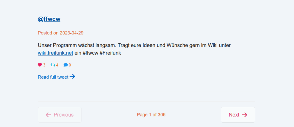
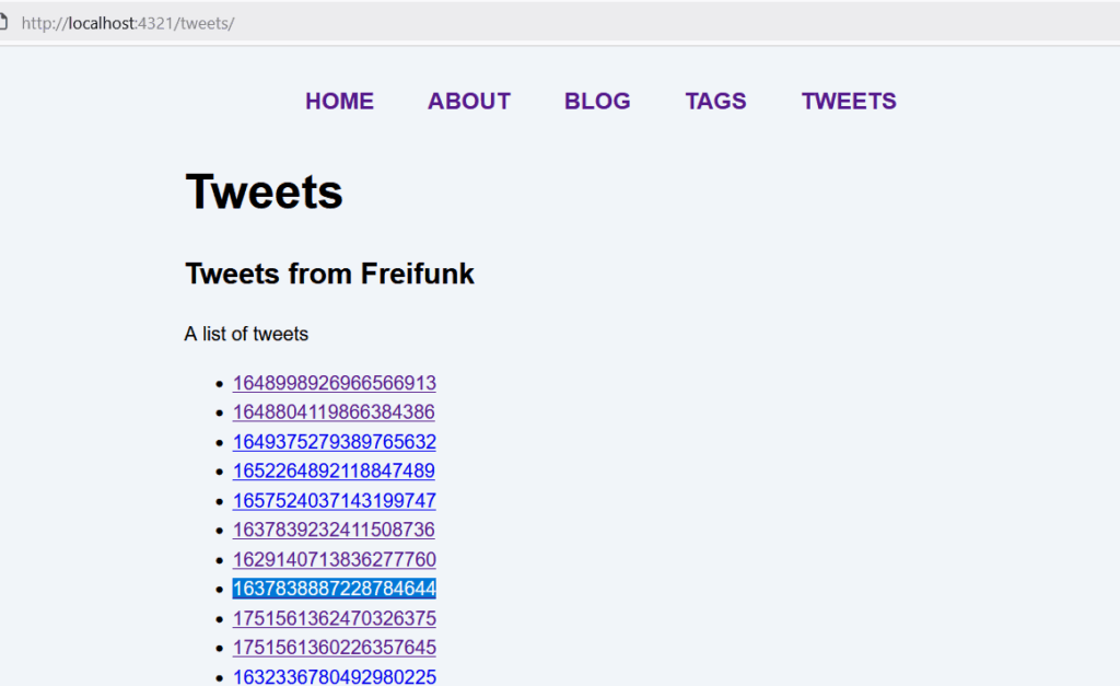
I’m so proud and excited to be writing this final blog post for Freifunk and to share what I’ve accomplished during GSoC 2025. It feels great to say that I’ve completed the main goals of the project—building a working Social Media Archive for Freifunk’s exported Twitter data. Here’s a quick rundown of the progress I’ve made this summer.
Milestone Highlights – All Goals Completed
Select the Static Site Generator (SSG) – Analyzed several existing technologies and decided on Astro as our SSG.
SSG Setup– Embraced learning web development for the first time and followed several tutorials to make my first static site using Astro. After this foundation, I reviewed the current state of the Twitter data fields and planned how this information would be extracted from the database.
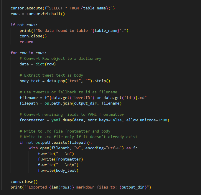
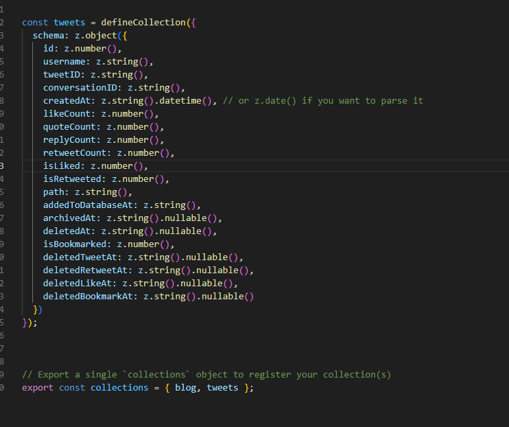
Develop Data Extraction Tool – Created a script to extract relevant fields from the archived SQLite3 database and normalize them into a unified schema.
Create Static Site Mockup – Generated an initial static website, but now combined it with the parsed and structured Twitter data.
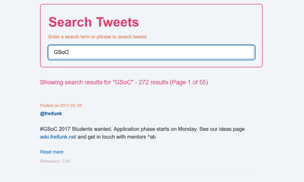
Implement Client-Side Search – Upgraded the website features further by adding client-side search functionality by preprocessing and indexing data during the build process.
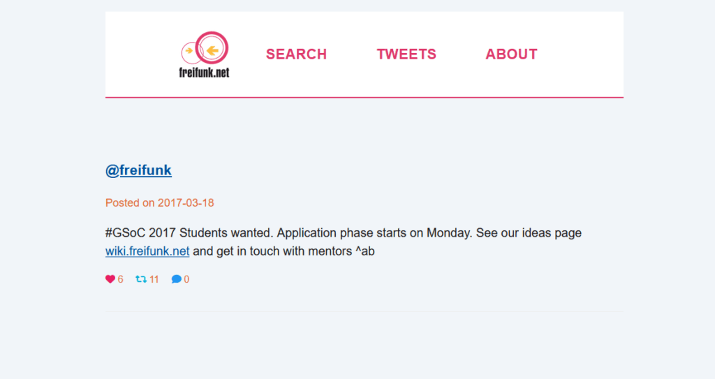
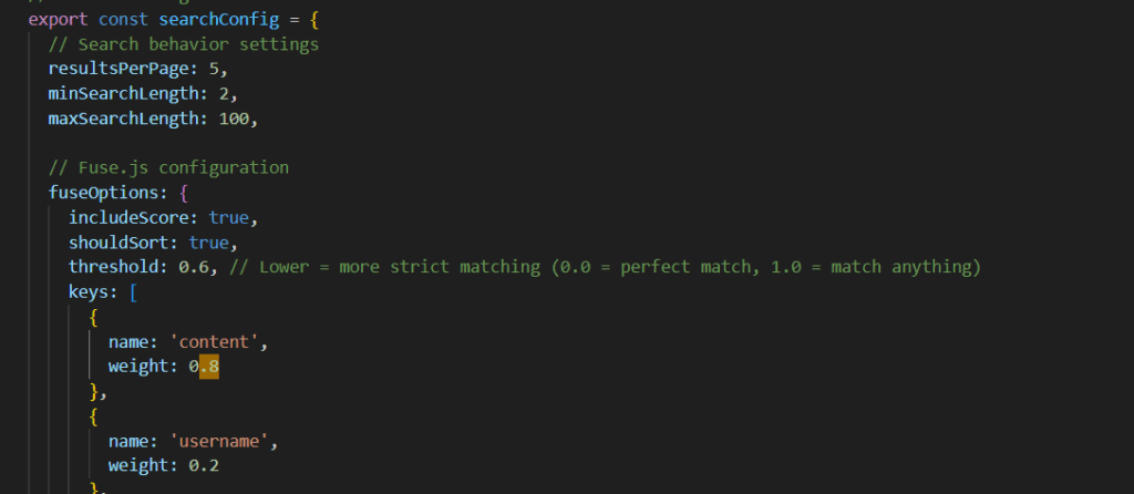
Customizable Theming Support – Designed the Social Media Archive with an easily customizable theme so others can adapt it for their own projects, while keeping Freifunk’s iconic pink this final version to reflect their identity.
Documentation and Deployment – Wrote comprehensive documentation on GitHub explaining how the Social Media Archive works. Also created a separate README for the build process to guide users through prepping the data for use on the site. Lastly, we deployed the website.
Test, Optimize, and Ensure Scalability – Tested the site using the full tweet database to ensure performance stayed solid. Also optimized the website build process to improve time complexity, making the SQL-to-Markdown extraction faster.
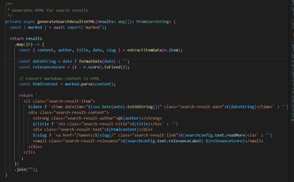
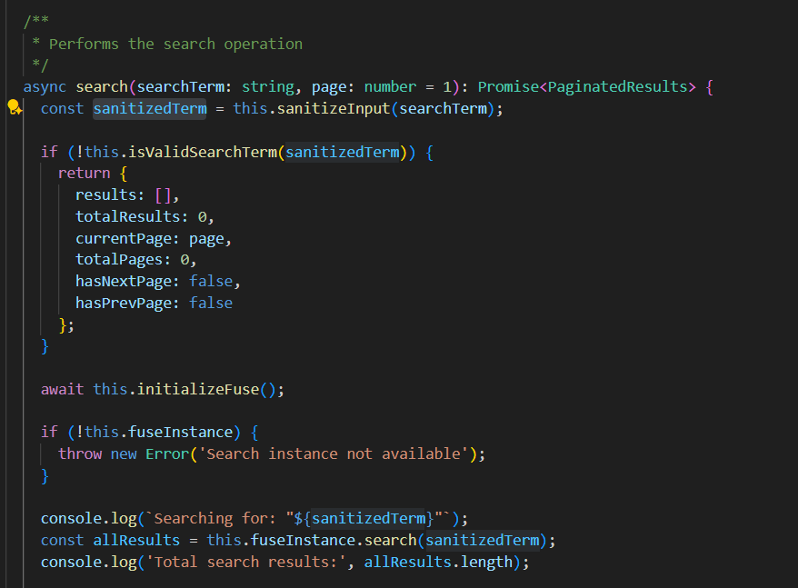
TypeScript code for rendering search results in HTML
Defining the relative weight of the content and username attributes to improve the relevance of search results
Using DOMPurify to sanitize user input while using the search functionality
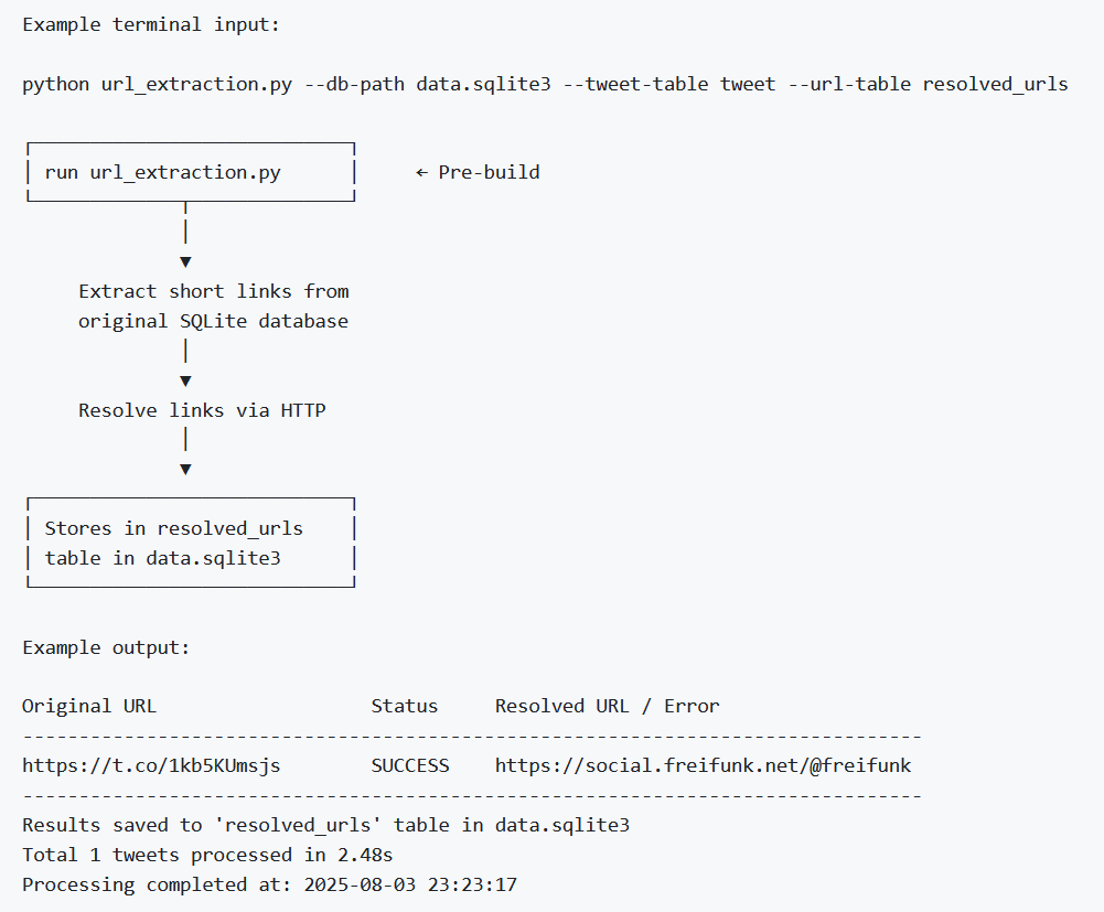
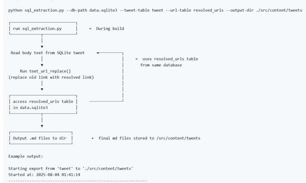
Refining the SQL to Markdow data extraction tool:
Part 1 documentation: The flow of the data extraction build scripts
Part 2 documentation: The flow of the data extraction build scripts
Remaining Work
Backend refactoring changes could be made to simplify the codebase. As this is my first attempt at web development, it’s likely not everything I did was as efficient as it could have been
Advancing the Search functionality so that the user can perform more sophisticated queries, like searching via “AND” keywords or by date.
Improving the organization of pages. For example, the Search page should be moved from the index.astro (home) page and replaced with the Tweet page
Challenges & Lessons Learned
I learned that web development is complex—there are many moving parts, tools, and dependencies, and plenty of opportunities for things to go wrong. Yet despite the challenges, it was also incredibly empowering. I was able to transform raw Twitter data stored in an SQL database into a browsable, visual archive. Seeing that transformation come to life was both rewarding and inspiring.
I also came to better understand the realities of working and learning remotely, particularly across significant time zone differences. Asynchronous collaboration can make it harder to stay aligned with teammates, so it’s important to schedule occasional synchronous check-ins to reconnect, clarify goals, and regroup.
Finally, I learned the importance of giving yourself more time than you think you’ll need. Things rarely work perfectly on the first (or even second) attempt. Building in extra time, staying patient, and approaching debugging with a calm, methodical mindset proved crucial to making steady progress.
Conclusion
I’m glad I decided to apply for GSoC back in March. This summer, I experienced real growth and learned many valuable lessons. I’m especially grateful for the generous support from my mentor, Andreas Bräu, the other contributors, and the GSoC and Freifunk communities. GSoC is a fantastic opportunity, and I would highly encourage others to apply.
I’m looking forward to continuing my contributions to the Social Media Archive in the future.
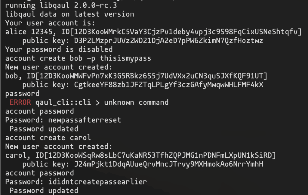
Hi everyone! As we reach the midpoint of Google Summer of Code 2025, I’m excited to share the progress no my project: qaul RPC User Authentication Layer. Working on the project has been challenging as well as rewarding for me, and I’m very excited to share what I’ve accomplished so far and what is still left.
Where are we
Core Password Management Implementation
I have built the foundational password management system within libqaul. This involves several key components.
Secure Password Hashing: I initally implemented hashing using bcrypt but after careful consideration, I migrated to Argon2.
Protobuf Integrations: Extend qaul’s existing RPC communication structure by adding new auth modules.
Updated the configuration framework to secure handle password hashes and auth settings, so that sensititve data is properly stored while maintaing compatibility with existing systems.
Authentication Module Development
The auth system is now integrated into libqaul’s arhitecture.
RPC Message Handling: Implemented comprehensive message processing for authentication requests and responses, including proper error handling and status reporting.
Challenge response: developed a secure authentication flow that uses cryptographic challenges rather than direct password transmission. This approach ensures that passwords neer traverse the network, and no two hash (that node use to verify password) are same due to different nonce for each authentication request. The structure for messages are below:
The larger picture for us is to create an infrastructure where we could enable multi-user per ndoe support, and web-based interface. Therefore we would be working on Session token management system that would validate the authenticated operatings and enable stateful user sessions while maintaining security.
Challenges
RPC system extension. Integrating authentication into qaul’s existing rpc infrastructure was a bit challenging for me initially, but a few wrong attempts gave me a clear picture. Also, the existing code helped me understand how things were working.
We wanted the user password to be actually very secure, so instead of simply hashing it, we now hash the user password with salt, let’s say hash1 and then libqaul send you a nonce, and using hash1 and nonce we calculate the hash2. This ensures that the hash2 is never the same for any existing passwords.
Next Steps
For the remainder of the project, I plan to focus on:
Session Management Completion
CLI Integration
Encryption Implementation
Conclusion
The midterm point helped me reflect on my journey, and I’m glad to say that the project is shaping up excellent. Wit the core authentication infrastructure completion and properly integration into libqaul. we have a solid foundation for secure multi-user support and future interface development. Thank you to my mentor Mathjud and the entire qaul community!
Hello everyone! As we reach the midpoint of Google Summer of Code 2025, I’m excited to share the progress on my project, Deep Q Network-based Rate Adaptation for IEEE 802.11ac Networks. The goal of this project is to build an intelligent rate control mechanism that can dynamically adapt transmission rates in Wi-Fi networks using Deep Reinforcement Learning. So far, I’ve implemented a basic DQN-based agent with a simplified environment, introduced group-based rate handling inspired by Minstrel_HT, incorporated success probability tracking, and collected real-world data using a shielding box. This post will walk through these key developments, the challenges encountered, and the next steps toward building a more robust and generalizable solution.
Background
Rate adaptation in Wi-Fi is a critical task that selects the most suitable Modulation and Coding Scheme (MCS) index for transmission. The MCS index encapsulates key physical-layer parameters such as modulations type, coding rate, bandwidth(BW), guard interval (GI), and a number of spatial streams (NSS). Traditional rate adaptation algorithms often rely on heuristics or statistical measurements to infer the best MCS under varying channel conditions.
In this project, we aim to explore a Deep Q-Network (DQN) based approach for intelligent rate adaptation. Rather than relying on predefined rules, the agent learns to select the optimal MCS indices by interacting with the environment and receiving feedback on transmission success and failure. Unlike many prior works focused solely on simulations, our primary aim is to integrate this learning framework with real-world experimentation using ORCA (Open-source Resource Control API). This enables us to evaluate learning-based adaptation in actual 802.11ac Wi-Fi environments. For more detailed background and motivation, please refer to my initial blog post. Please check out my initial blog post for more information.
1. What We’ve Accomplished So Far
1. Initial Setup -DQN with Dummy States
In the early phase of the project, a basic DQN agent was set up with a placeholder environment to validate the training pipeline. The agent was designed to choose among discrete actions (initially up/down rate shifts), but the state representation was simplified to dummy values.
Each state was initially defined as the list of Received Signal Strength Indicator (RSSI), Signal Noise Ratio(SNR), transmission successes, retransmission attempts, and current MCS (among 8 fixed MCS values). This served as a proof-of-concept to validate the learning loop of DQN interacting with a Gym-style environment.
This served as a proof-of-concept to validate the learning loop of a Deep Q-Network (DQN) interacting with a Gym-style environment. This environment follows the OpenAI Gym(reference) interface, where an agent observes a state, takes an action, and receives a reward and next state in return. This setup helps modularize the environment and makes it easier to test and evolve reinforcement learning agents systematically.
2. Design of the DQN-Based Rate Adaptation Algorithm
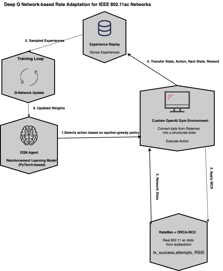
In this section, we outline the overall system architecture of our Deep Q-Learning-based Rate adaptation framework. The goal is to give a clear block-level understanding of how the components interact, followed by an explanation of key choices around state, action, reward, and the agent.
Below is the high-level block diagram of the DQN-based rate adaptation system.
Fig1. Current Implementation
PyTorch was chosen as the deep learning framework as it offers easier debugging and flexibility compared to static graph libraries like TensorFlow 1.x. The API is clean and beginner-friendly. As PyTorch is widely used in reinforcement learning research, the community support is strong, which makes it easier to find references and extend the work if needed.
Components of the DQN
1. Q-Network
A simple feed-forward neural network that takes the current state as input and outputs Q-values for each possible action (rate group). This helps to estimate how good each action is from the current state.
2. Target Network
To stabilize training, we maintain a separate target Q-network that is periodically synced with the main Q-network.
3. Custom Gym Environment A tailored environment was built following the OpenAI Gym interface to simulate the Wi-Fi rate adaptation scenario.
The state includes variables like RSSI, current rate index, number of attempts, and success history.
The action space corresponds to selecting among a defined set of MCS rates.
The step function computes the resulting throughput, success, and termination condition based on real trace data.
4. Agent
The component is responsible for selecting actions using an epsilon-greedy strategy, balancing exploration and exploitation during learning.
5. Experience Replay Buffer
Transitions (state, action, reward, next_state) are stored in a fixed-size buffer. During training, a batch of past experiences is randomly sampled to break temporal correlations of sequential experiences and improve sample efficiency.
6. Epsilon-Greedy Exploration Strategy
To balance exploration and exploitation:
Initially, the exploration rate is set to 100%. This means the agent will select the random actions(rates) to determine which give better rewards.
The exploration rate is decayed linearly to promote exploitation (select the best known action) in the later stages.
7. Training Loop and Episode Tracking
The agent was trained over a series of interactions with the environment using a well-structured training loop, which mimics how reinforcement learning systems learn from trial and error.
In our setup:
An episode is a complete cycle of interaction between the agent and the environment. It starts with an environment reset and continues until the agent reaches a terminal state (e.g retransmissiion threshold, low success rate), or the maximum allowed steps for the episodes are completed.
A run refers to one complete training session, which in our case consists of 500 episodes. We can repeat runs with different random seeds or hyperparameters for comparison.
Each episode proceeds step-by-step, where the agent:
Selects an action (rate) using an epsilon-greedy policy.
Takes the action in the environment and receives the next state, reward, and a termination flag.
Stores the transition (state, action, reward, next_state, done) in the experience replay buffer.
Samples a batch from the buffer to update the Q-network using the Bellman equation.
Synchronizes the target network with the policy network at fixed intervals.
This structure enables stable learning over time, leveraging both exploration and exploitation.
Fig2. Sample Training Behavior
2. Core DQN Logic: State Design, Reward & Group-Based Adaptation
As we transitioned toward real-world deployment of our DQN-based rate adaptation agent using ORCA, we faced a key practical constraint: Signal-to-Noise Ratio (SNR) is not directly available from the ORCA interface. This led to a redesign of the agent’s input state and reward function, grounding our system in metrics that are actually observable in real Wi-Fi environments.
a. Removal of SNR
In early versions of the environment, SNR was included as part of the agent’s observation space. However, since ORCA (the testbed we use for data collection and deployment) does not expose SNR, it cannot be used in real training or evaluation. As a result:
We removed SNR from the environment’s observation space.
Instead, we rely on RSSI (Received Signal Strength Indicator), which can be collected reliably from transmission feedback logs in ORCA.
In the simulation, RSSI is initialized at –60 dBm and updated with small noise in each step. In real training, RSSI will be sourced directly from logs collected during hardware tests.
b.State Definition
Each state observed by the DQN agent is a 4-dimensional vector:
current_rate: The transmission rate index selected by the agent in the previous step.
rssi: Signal strength (used instead of SNR), simulated in the dummy setup and real in actual experiments.
tx_success_rate: Maintains an exponential moving average of recent transmission outcomes.
tx_retransmissions: Counts retransmissions, capped at 10.
This formulation provides a minimal yet sufficient summary of recent channel behavior and agent action history.
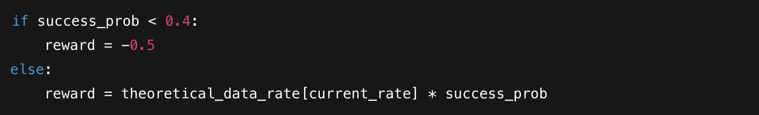
c. Reward Calculation
The reward is designed to reflect actual performance, balancing success and throughput:
success_prob is computed as:
Success_prob = successes/attempts
If the success probability for a rate is too low (<0.4), the agent receives a penalty.
Otherwise, the reward scales with the theoretical data rate of the selected rate and its current success probability.
d. Attempt and Success Counts
The environment internally tracks the number of transmission attempts and successes per rate using two dictionaries:
On each action step, the environment:
Increments the attempt count for the selected rate.
Samples a binary transmission outcome using the current estimated success probability.
Updates the success count if the transmission succeeded.
e. Why Warm-Start the Attempt and Success Counts
At the start of training, all rates have 0 attempts and 0 successes. This makes success probability undefined or zero, which results in poor early rewards and unstable learning.
To mitigate this, we use a warm-start strategy:
A few rates are preloaded with 5 attempts and 4 successes.
This gives the agent initial traction and prevents early negative feedback loops.
This trick significantly stabilizes training in the first few episodes and is especially useful when rewards are sparse or noisy.
f. Group-Based Rate Adaptation (Inspired by Minstrel_HT)
In our implementation, we adopted a group-based rate adaptation strategy inspired by the structure used in Minstrel_HT and aligned with the rate grouping logic defined within ORCA. Each group corresponds to a specific combination of key physical-layer parameters, including spatial streams(NSS), bandwidth, guard interval, MCS modulation and coding.
Rate grouping is employed to generalize success estimates across similar rates.When a rate has never been used (0 attempts), its success probability falls back to that of higher-used rates in the same group.For example, our project uses Group 20, which corresponds to 3 spatial streams, 40 MHz bandwidth, and a short guard interval (SGI). The associated rate indices and their characteristics are:
Rate Index
MCS
Modulation
Coding
Data Rate (Mbps)
Airtime (ns)
200
BPSK, 1/2
BPSK
1/2
45.0
213,572
201
QPSK, 1/2
QPSK
1/2
90.0
106,924
202
QPSK, 3/4
QPSK
3/4
135.0
71,372
203
16-QAM, 1/2
16-QAM
1/2
180.0
53,600
204
16-QAM, 3/4
16-QAM
3/4
270.0
35,824
205
64-QAM, 2/3
64-QAM
2/3
360.0
26,824
206
64-QAM, 3/4
64-QAM
3/4
405.0
23,900
207
64-QAM, 5/6
64-QAM
5/6
450.0
21,424
208
256-QAM, 3/4
256-QAM
3/4
540.0
18,048
209
256-QAM, 5/6
256-QAM
5/6
600.0
16,248
Fig3. Details of Group 20
g. From Incremental Actions to Direct Rate Selections
Initially, the action space consisted of just 2 actions: increase or decrease the rate(MCS-style adaptation). However, after several trials it was clear that this incremental strategy was too slow, and most supported rates were never reached during the training.
For a simple start, we chose 10 rates out of all the supported rates.
So, we updated the action space to be direct rate selection:
Instead of navigating one rate at a time, the agent now chooses directly from a subset of these 10 representative rates.
This allows faster exploration and better convergence.
This change made a major difference in the agent’s ability to adapt and explore diverse transmission configurations.
3. Real Data Collection with Shielding Box
To enable rate adaptation in real-world Wi-Fi networks, we began by collecting real channel data using controlled hardware setups. This data is essential for grounding our DQN training in reality and ensuring the learned policy performs well in practical deployment.
Rather than relying solely on simulated environments, our aim is to train and evaluate the DQN algorithm on actual wireless conditions. This is crucial for developing a rate adaptation mechanism that is robust and effective in real network scenarios.
Test Setup
We used a shielding box setup to ensure accurate and isolated measurements. The shielding box allowed us to eliminate external interference, offering a reproducible environment to study channel behavior. ORCA provided fine-grained control over the STA, such as adjusting MCS rates, attenuation and collecting relevant metrics
Measurement Scope:
We systematically tested the full set of supported transmission rates to understand their performance under varying signal conditions:
Covered all supported rates (hex:120 to 299)
Grouped rates into prefix-based clusters (e.g., 12, 40)
Each group was tested across attenuation levels from 40 dB to 70 dB in 5 dB steps for 20 seconds in each step.
For each group, we collected:
RSSI over time
Selected transmission rates
Corresponding throughput
These metrics were then visualized in the form of plots to understand behavior patterns and build insights.
The real-world dataset will be instrumental in training the DQN agent directly on real channel traces. We can validate the reward function logic and evaluate the effectiveness of the learned rate adaptation policy with this data. Finally, it will be helpful in deploying and testing the trained policy in live networks.
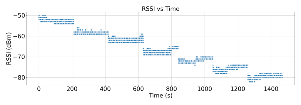
For Group 20 => Rates 200-209(Hex) (Fig3.)
Fig4. RSSI vs Time
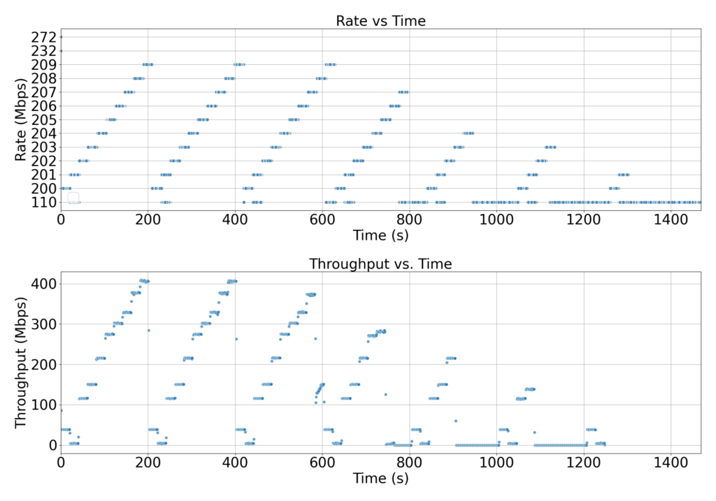
Fig5. Rates and Corresponding Throughput vs Time
So far, the environment simulated RSSI dynamics using random noise, which lacks the variability and structure of real wireless channels. Moving forward, this collected dataset opens the door to a more realistic simulation and training loop, such as:
Conditional sampling: RSSI values and throughputs can be sampled based on selected rate and attenuation level, simulating how a rate would realistically perform under current channel conditions.
Replay of real RSSI traces: Instead of generating random RSSI values, the environment can replay actual RSSI sequences from the logs.
Rate-Throughput mapping: Instead of assigning theoretical data rates(Mbps), we can use empirical throughput measurements for each (rate, RSSI) pair, making the reward signal much more grounded.
Conditional sampling: RSSI values and throughputs can be sampled based on selected rate and attenuation level, simulating how a rate would realistically perform under current channel conditions.
This integration would make the environment closer to real-world performance, enabling the agent to learn from more structured feedback.This is a critical step for bridging the gap between simulation and real deployment.
4. Next Steps
Environment Refinement Using Real Data
Use the collected shielding box data to model real rate-to-reward mappings.
Replace random assignment of noise and RSSI values with the real trace data.
Train with Full Action Space
Expand action space from binary (up/down) to direct rate selection.
Evaluate trade-offs in convergence speed and learning stability. –
Integration with ORCA and Real Hardware
Plug the DQN model into the ORCA framework for live experimentation.
Use real-time stats from RateMan to drive the agent’s decisions.
Logging & Visualization
Visualize Q-values, state evolution, and rate changes over time. Add detailed logging of action-reward-history.
5. Challenges and Open Questions While progress has been substantial, several challenges and open questions remain, which need thoughtful solutions going forward:
1. Kickstarting Learning Without Warm-Up Rates
To prevent the agent from receiving only negative rewards in early episodes, we manually pre-filled success/attempt stats for certain rates. However, in real deployments, such a warm-up is not always possible.
Challenge: How to design exploration or reward shaping mechanisms that allow agents to learn from scratch without manual initialization?
2. Large Action Space: Curse of Dimensionality
The supported rates in our setup are ~232. A large action space may:
Make learning slower and unstable
Lead to sparse exploration and poor generalization
Cause overfitting to rarely used or unreachable rates
3. High Attenuation Handling
Under higher attenuation (e.g., 65–70 dB), only lower MCS rates may be feasible.
Challenge: Should the agent learn rate-attenuation mappings and restrict its actions contextually, or penalize high-rate selections under weak channel conditions?
4. Real-Time Constraints
The agent needs to make decisions at frame-level or sub-second intervals. Any delay in inference or policy selection may render the decision obsolete due to fast-varying wireless environments.
Challenge: Can we compress or distill the trained agent for low-latency environments?
Conclusion
The first half of GSoC has been a learning-intensive and productive phase. From environment design to agent training, we now have a complete pipeline to simulate, train, and evaluate DQN-based rate adaptation. The next steps will focus on making the model robust, interpretable, and hardware-ready.
Please feel free to reach out if you’re interested in reinforcement learning in networks or Wi-Fi resource control. Thank you for reading!
References
1. Pawar, S. P., Thapa, P. D., Jelonek, J., Le, M., Kappen, A., Hainke, N., Huehn, T., Schulz-Zander, J., Wissing, H., & Fietkau, F.
Open-source Resource Control API for real IEEE 802.11 Networks.
2. Queirós, R., Almeida, E. N., Fontes, H., Ruela, J., & Campos, R. (2021).
Wi-Fi Rate Adaptation using a Simple Deep Reinforcement Learning Approach. IEEE Access.
Userspace programs fires a command that interacts with wifi : programs such as `iw`, `hostapd`, `wpa_supplicant` etc.
Command is passed to the kernel through _nl80211_ over the netlink protocol, in openwrt it is usually handled by [tiny-libnl](https://git.openwrt.org/?p=project/libnl-tiny.git)
_cfg80211_ is here to bridge the userpace and the drivers so that with nl80211 they provide a consistent API, it’s also here that parts of the regulatory spectrum use is enforced depending on country specific legislation.
_mac80211_ then provides a software implementation of wifi behaviors such as queuing, frame reordering, aggregation, mesh support etc.
The driver (ath9k or *mac80211_hwsim*) then handles hardware specificities
Why is this important for our project
This layered approach is essential to our project, as it will enable us to create virtual tests beds that should be almost transparent to a real world experiment.
By just simulating the last brick – mac80211_hwsim – we’ll be able to recreate the whole wifi stack. We will still see the same exact path consisting of : userspace configuration -> nl80211 -> cfg80211 -> mac80211
Which means that without the need for expensive and complicated set up, we achieve the same possible tests for configuring the different interfaces, and in our case with the added reproducibility : setting up the infrastructure will only require a computer able to launch qemu-system, and if we decide to reproduce it with real hardware, we should observe an almost 1:1 reproducibility of the tests.
Virtualizing wifi : many tools, troubling setup
So we now that we have a clearer understanding on how wifi is handled in the Linux Kernel, and the existence of a tool to simulate wifi hardware, let’s see what is possible to do with it !
mac80211_hwsim in LibreMesh ?
Since LibreMesh is built on OpenWRT, our first task will be to bring mac80211_hwsim to OpenWRT.
Thankfully, this tool is known and already used by the OpenWRT community, and it is delightfully provided as a package that you can install in your system through opkg : opkg install kmod-mac80211-hwsim Which means, no need for custom kernel setup and compilation – and that’s good news.
Installation methods :
If your machine has an AMD/Intel CPU, simply go get the combined (squashfs) of the Generic x86/64 through the firmware selector.
unzip the image : gunzip openwrt-*-x86-64-generic-squashfs-combined.img.gz
You should then end up with something like that :
openwrt-24.10.2-x86-64-generic-squashfs-combined.img Simply put, this is a kernel+root file system (that’s what combined means), using a compressed read only filesytem (squashfs).
Now we need to instantiate our virtual machine, using qemu it can be done like this :
Just wait a bit for the boot to finish, you should see a Please press Enter to activate this console.
Inside the vm you’ll then have to run : uci set network.lan.proto='dhcp'
uci commit network
service network restart
Inside the vm you’ll then have to run : uci set network.lan.proto='dhcp' uci commit network service network restart
This convert the LAN to a DHCP client and allow the VM to grab the 10.0.2.x lease from QEMU, Which will then enable you to run : opkg update
and finally : opkg install kmod-mac80211-hwsim
By default, mac80211_module is loaded with 2 radios, but the behavior can be changed with this command : insmod mac80211_hwsim radios=X` with X the number of radios you want to have in your VM.
Let’s also not forget to include the right packages since we want to test wifi : Since we’re not constrained by flash space on our laptop/computer, we’ll use wpad : opkg install wpad
Congratulation, you now have an OpenWRT based virtual machine with a working virtual wifi ! Actually, not so fast…
One of the classical example when searching for the documentation regarding mac80211_hwsim module is the access point/station association using two different virtual radios (on the same host). 12 So let’s be original, and recreate this example (but in this case in OpenWRT !).
Virtual AP/Station association in a OpenWRT virtual machine :
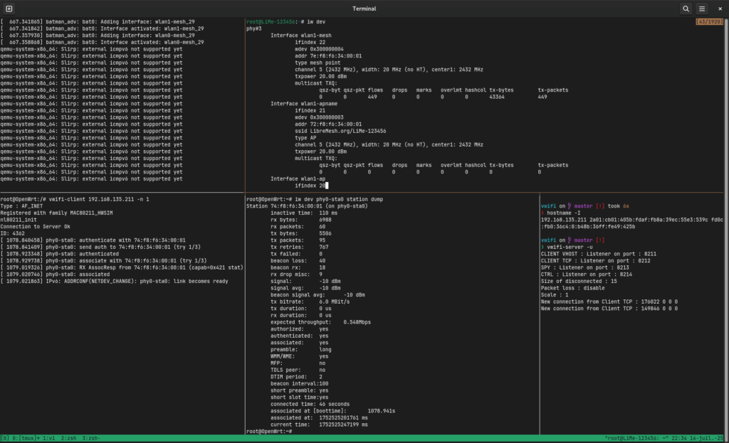
When we install mac80211_hwsim/boot the VM, it should auto load the module with 2 radios. You can check the presence of the 2 radios with this command :
As for the wifi devices, so far, nothing : iw dev won’t return anything at this point. We now need to configure these two (virtual) physical radios in order to have : an AP and a station. Let’s check the default configuration of the wireless in our image :
As we can see, both of our wifi-device are disabled, and also both in ap mode. So the easy way out of this would be to do : uci set wireless.radio0.disabled=0
uci set wireless.radio1.disabled=1
uci set wireless.radio1.mode=sta
uci commit
wifi reload
With all that we should be set ? No ? Still nothing. This was a real mystery for me, but after some digging, it appears that when using the 6g band, wpa3 is mandatory. This is defined by the IEEE 802.11ax standard, and in our case the wifi 6E extension. Since encryption testing isn’t on the scope of this project so far, let’s be conservative and try some true and tested wifi bands (2g) and see what happens.
In the end your /etc/config/wireless should look something like that :
config wifi-device ‘radio0’ option type ‘mac80211’ option phy ‘phy0’ option band ‘2g’ option channel ‘1’
With this configuration you still need to wifi reload or reboot if you don’t see any changes happening. We finally have our prized AP/station association :
daemon.notice hostapd: phy0-ap0: interface state UNINITIALIZED->ENABLED daemon.notice hostapd: phy0-ap0: AP-ENABLED daemon.notice wpa_supplicant[1825]: phy1-sta0: SME: Trying to authenticate with 02:00:00:00:00:00 (SSID=’OpenWrt’ freq=2412 MHz) daemon.info hostapd: phy0-ap0: STA 02:00:00:00:01:00 IEEE 802.11: authenticated daemon.notice wpa_supplicant[1825]: phy1-sta0: Trying to associate with 02:00:00:00:00:00 (SSID=’OpenWrt’ freq=2412 MHz) daemon.info hostapd: phy0-ap0: STA 02:00:00:00:01:00 IEEE 802.11: associated (aid 1) daemon.notice hostapd: phy0-ap0: AP-STA-CONNECTED 02:00:00:00:01:00 auth_alg=open daemon.info hostapd: phy0-ap0: STA 02:00:00:00:01:00 RADIUS: starting accounting session 2E622F6D18713536 daemon.notice wpa_supplicant[1825]: phy1-sta0: Associated with 02:00:00:00:00:00 daemon.notice wpa_supplicant[1825]: phy1-sta0: CTRL-EVENT-CONNECTED – Connection to 02:00:00:00:00:00 completed [id=1 id_str=] daemon.notice wpa_supplicant[1825]: phy1-sta0: CTRL-EVENT-SUBNET-STATUS-UPDATE status=0
Let’s check what iw is reporting :
iw dev phy#1 Interface phy1-sta0 ifindex 7 wdev 0x100000002 addr 02:00:00:00:01:00 type managed channel 1 (2412 MHz), width: 20 MHz (no HT), center1: 2412 MHz txpower 20.00 dBm multicast TXQ: qsz-byt qsz-pkt flows drops marks overlmt hashcol tx-bytes tx-packets 0 0 0 0 0 0 0 0 0 phy#0 Interface phy0-ap0 ifindex 8 wdev 0x2 addr 02:00:00:00:00:00 ssid OpenWrt type AP channel 1 (2412 MHz), width: 20 MHz (no HT), center1: 2412 MHz txpower 20.00 dBm multicast TXQ: qsz-byt qsz-pkt flows drops marks overlmt hashcol tx-bytes tx-packets 0 0 11 0 0 0 0 1358 11 And finally : iw dev phy0-ap0 station dump Station 02:00:00:00:01:00 (on phy0-ap0) inactive time: 4950 ms rx bytes: 2077 rx packets: 50 tx bytes: 131 tx packets: 2 tx retries: 0 tx failed: 0 rx drop misc: 0 signal: -30 dBm signal avg: -30 dBm tx duration: 0 us rx bitrate: 54.0 MBit/s rx duration: 0 us authorized: yes authenticated: yes associated: yes preamble: short WMM/WME: yes MFP: no TDLS peer: no DTIM period: 2 beacon interval:100 short preamble: yes short slot time:yes connected time: 1232 seconds associated at [boottime]: 59.854s associated at: 1752513660712 ms current time: 1752514892128 ms
All in all, lots of troubleshooting, qemu-system network was a bit novel for me and I spent a lot of time on it figuring it out why some things worked on others didn’t. Also having mac80211_hwsim fully working in a OpenWRT qemu vm was definitely not easy at first : some documentation for the setting it up in a regular Linux environment, but didn’t find much regarding OpenWRT ?
Enabling mac80211_hwsim in LibreMesh
Now that we have a proof of concept of virtual wifi working in OpenWRT, let’s port it to LibreMesh.
‘kmod-mac80211-hwsim wpad` to the firmware selector (getting opkg to work in a Libremesh vm is a bit tricky – doing like so is a lot easier)
request a build
then you’ll be able to recreate the steps from the last section to have AP and mesh radios (You should be able to see the mesh interfaces connect to each other if put on the same channels)
On a custom build
Now that we mostly have figured out mac80211_hwsim with a generic image, let’s enable it in a custom LibreMesh build.
By following these instructions you should be able to get mostly there.
using make menuconfig, you will need to select these targets :
Target System : x86 Subtarget : x86_64
Then it will simply selecting the specific libremesh packages, and lastly :
Save your config in .config, compile it make -j$(nproc) and then you’ll find your different images in bin/targets/x86/64.
Setting up mac80211_hwsim will require the same steps as the last two (setting the right band/channels/radio)
Conclusion of mac80211_hwsim in Libremesh
In the end mac80211_hwsim provides an excellent tool to test different wifi configuration, enabling it in a LibreMesh build is pretty straight forward, but as for OpenWRT stock image t requires a bit of manual work to set everything right.
My trials and errors for enabling mac80211_hwsim in Libremesh led me to discover some undefined behavior in LibreMesh when the firmware interacts with a wifi 6E able radios, which I will need to provide a patch for in order to continue my integration of qemu wifi testing to LibreMesh in the next half of my GSOC.
VM to VM communication using wifi
I’m proud to announce that I’ve finally managed to recreate the AP-STA scenario using two differents QEMU virtual machines ! OpenWRT <-> OpenWRT as well as LibreMesh <-> OpenWRT was possible. Once I’m able to fully control it and document it, I will provide a libremesh-profile with and easy setup.
This experiment relies on the vwifi project which comes in two part :
vwifi-server which will run on the host and is here to provide a medium for our wifi : in its default config, it will broadcast the wifi frames of the client connected to it to the other clients.
vwifi-client that will run on the guest : it basically relies on mac80211_hwsim to create real wifi frames, then relay them to the vwifi-server it is connected to. It also receives wifi frame from the others clients through the server, and manage to inject them in the VM wifi stack, so they get treated correctly and connection is possible.
Building the project is well documented in the README, and one advantages of this project is that it is OpenWRT compatible if we follow closely the instructions.
I struggled a lot a first, thinking I should cross compile it against my custom LibreMesh build, but it seems that as long as you get the right SDK you shouldn’t encounter any issues, aside from the usual qemu troubleshooting.It is also possible to build vwifi-client in order for it to work with vhost-vsock instead of TCP, but I so far didn’t manage to do that/didn’t test it right.
Caveats
run the vwifi-server like this : vwifi-server -u this will prevent overlapping in the mac address when relaying to the other clients, and save you some time figuring out what’s really happening.
When copying the vwifi-client file to the guest, use these options : scp -O -p <forwarded port> root@127.0.0.1 since otherwise it will try to rely on sftp, which might not be installed on the OpenWRT guest VM.
vwifi-client needs to connect to the host : use the IP from hostname -I. Inside the VM you need to run something like that : `vwifi-client -n –mac
If you don’t want to set it up as a service, remember that you need to remove the mac80211_hwsim module, then insert it again but with 0 radios : insmod mac80211_hwsim radios=0
In LibreMesh, the current default wireless config is broken, a patch is coming very soon that will allow a seamless integration with the testing, but so far lime-config will put each radios advertised by mac80211_hwsim in the 6g band channel 48 : this won’t work, you need to manually change it to have (modify the /etc/config/wireless)
I still need to provide a full guide and scripts on how to recreate the experiment, but with this picture you should see what it is expected to have :
You can see on the top the LibreMesh VM acting as the access point, with on the left the serial interface running vwifi-client and on the right an ssh connection to this VM used to manage it. At the bottom of the image it is the same setup but using a different VM, this time with a regular OpenWRT image, acting as the station. We can clearly see the station being connected to the AP from a the other VM.
Integration with LibreMesh testing ?
My initial tests and discoveries with virtualized wifi in a QEMU environment and the different tools that this kind of setup enables makes me more and more confident in the usefullness of adopting this approach for future development in LibreMesh and OpenWRT. From this 6 weeks coding period that were mostly troubleshooting and figuring why things don’t work I’ve managed to find an undefined behavior in the way LibreMesh sets itself up on newer hardware without the need to acquire the said hardware, it also seems that it’s not even been discovered yet by an user : fixing bugs before they even show up.
Now for integrating this kind of qemu testing, the LibreMesh community have decided to use the openwrt-tests framework, a framework based on labgrid aimed at providing ways to write and run tests for OpenWRT devices, being real hardware or virtual one (in our case).
I’ve already made some preliminary work for enabling LibreMesh to integrate with this framework. So far the framework provide satisfaction with my goals, the only real issues I’ve encountered were actually the divergence between OpenWRT and LibreMesh in some areas, meaning all the demos tests need some integration before being part of the testing pipeline.
Conclusion
I’ve mostly met my goal of having a working virtualized LibreMesh wifi mesh using a qemu infrastructure, I’m a bit behind regarding documentation as well as automation, but my plan is still well defined and I hope now mostly trouble free.
I now should be able in the coming weeks to :
Provide ample documentation for future work in this area
Leverage the new testing framework to provide reproducible and automated testing scenario, portable to real hardware
Fully integrate the project with LibreMesh testing pipeline, with documentation for extension
Port the current Docker based test to the new QEMU environment.
Bonus
I’ve had the pleasure to meet with the Freifunk/OpenWRT/LibreMesh community over the BattlemeshV17 organized in Sundhausen and I must say it was a very nice experience, learned a lot, flashed my first router with LibreMesh and more than everything felt very welcomed ! Thank you very much to the organizators and the participants, hope to see you again very soon.
This blog documents my ongoing progress with LibreMesh during Google Summer of Code (GSoC) 2025. Specifically, I’m focusing on integrating OpenWrt-native solutions and simplifying LibreMesh modules.
Currently, I am working on two main tasks:
Replacing deferrable-reboot with watchcat: Migrating LibreMesh’s custom reboot scheduling script to the built-in OpenWrt watchcat package for improved reliability.
Migrating DHCP functionality from dnsmasq to odhcpd: Transitioning DHCP and IPv6 handling to OpenWrt’s native odhcpd, currently in development and community testing.
For testing and validation, I’m using three physical routers configured to simulate realistic network conditions.
Task 1: Integrate OpenWrt’s watchcat via Hardware Detection
a. Motivation
The primary motivation for replacing LibreMesh’s deferrable-reboot script with OpenWrt’s watchcat is to leverage upstream-maintained tools, reduce redundancy, and enhance maintainability. watchcat provides robust functionality including scheduled reboots and network monitoring to automatically reboot routers in case of failure.
The design involves creating a hardware-detection (HWD) module within LibreMesh, enabling dynamic generation of watchcat configurations from user-defined UCI entries.
b. Implementation Details
The new package, lime-hwd-watchcat, is implemented in Lua, performing the following:
Unique Section Identification: Creates unique configuration section names prefixed with hardware identifiers to avoid conflicts.
Cleaning Up Configurations: Removes previously generated watchcat configurations.
Dynamic Configuration Generation: Reads entries from LibreMesh’s UCI configuration (hwd_watchcat) and generates corresponding /etc/config/watchcat entries.
Service Management: Automatically reloads watchcat after applying configuration changes using the /etc/init.d/watchcat reload command.
c. Testing & Validation
Testing involved:
Configuring custom UCI settings under config hwd_watchcat.
Validating automatic generation and updates to /etc/config/watchcat.
Confirming the proper removal of old configurations.
Checking watchcat service status and reload logs for expected behavior.
Default configuration:
Lets change it with the new package! Using:
uci add lime-node hwd_watchcat
uci set lime-node.@hwd_watchcat[-1].mode='ping_reboot'
uci set lime-node.@hwd_watchcat[-1].pinghosts='4.2.2.2'
uci set lime-node.@hwd_watchcat[-1].pingperiod='30s'
uci set lime-node.@hwd_watchcat[-1].period='6h'
uci set lime-node.@hwd_watchcat[-1].forcedelay='1m'
uci commit lime-node
And after using ‘lime-config’
d. Resources
You can see the code and the PRs for this package here:
OpenWrt’s native odhcpd daemon already powers IPv6 RA/DHCPv6 and integrates tightly with ubus. The goal is to phase out dnsmasq’s DHCP functionality in favor of odhcpd, leveraging its superior IPv6 support, integration with OpenWrt, and streamlined lease handling.
The new shared-state-odhcpd_leases package watches local leases, serialises them as CRDT objects via shared-state-async, and injects remote leases back into odhcpd, giving every node the same “view” of the network.
b. Implementation Details
The new package is entirely based in Lua. Its components fall into three small groups:
UCI defaults script (90_odhcpd-lease-share) – executed once at install time.
registers a community-scoped CRDT called odhcpd-leases, telling shared-state to refresh every two minutes and to expire entries after twenty;
sets two critical odhcpd options: leasetrigger points to our publisher script, and maindhcp='1' turns odhcpd into the sole DHCP server;
creates a legacy-friendly symlink /etc/ethers → /tmp/ethers.mesh;
finally reloads odhcpd so the new trigger takes effect.
Publisher (shared-state-publish_odhcpd_leases) – called by odhcpd whenever a lease changes. It fetches the current lease table with ubus call dhcp ipv4leases, distils it to the minimum JSON mapping IP → {mac,hostname}, and pushes that into the CRDT bus with shared-state-async insert odhcpd-leases.
Generator (shared-state-generate_odhcpd_leases) – executed on every CRDT update that the node receives. It writes the merged dataset to /tmp/ethers.mesh, moves the file atomically, and reloads odhcpd so the daemon immediately serves and announces the foreign leases as if they were local.
Unit tests live in tests/test_publish_odhcpd_leases.lua; they stub ubus, io.popen and os.execute to validate. The tests run in CI, so regressions in JSON shape or error handling are caught before merging.
c. Testing & Validation
The following testing methods are in progress:
Unit tests verify robustness of JSON serialization and shared-state publishing logic, covering normal, empty, and malformed market cases.
Deployment tests across three routers:
Confirm odhcpd takes over DHCP (uci show dhcp shows maindhcp=1).
Check presence and updates of /tmp/ethers.mesh and /etc/ethers symlink.
Simulate lease assignment and verify real-time propagation between nodes.
Service behavior:
Observe leasetrigger invocation on odhcpd-update.
Ensure stable operation over lease churn and node restarts.
So, for show how this works, I’ve two routers running LibreMesh, node-1 and node-2.
I connect a device in node-1, then I confirm it with ubus call dhcp ipv4leases '{}'
Then the publisher fires and odhcpd runs the shared-state-publish_odhcpd_leases script, which inserts the JSON blob into the CRDT bus.
Seconds later, on node-2 I dump the CRDT and see the same lease authored by node-1:
This is a minimal example, feel free to test anything you want!
d. Resources
Pull Request of the package,. Task 2 remains actively in development. Upcoming efforts will involve extensive community testing and careful analysis of how removing dnsmasq‘s DHCP functionality impacts related features and dependencies.
Reflection
The first half of the project required me to dive deeper into LibreMesh’s internals than initially expected, giving me a profound appreciation for this powerful mesh networking tool.
The most valuable lesson was recognizing that removing code (such as the deferrable-reboot script or dnsmasq’s DHCP logic) can be just as rewarding as adding new features. Simplifying the stack enhances its predictability and maintainability, ultimately benefiting the entire LibreMesh community.
Conclussion
After these two initial tasks, LibreMesh now:
Reboots through watchcat, an OpenWrt-native tool with LuCI support,
Serves and synchronizes DHCP leases via odhcpd and a lightweight CRDT-based sharing mechanism,
Incorporates automated tests to ensure reliability and stability through continuous integration (CI).
Looking ahead, I will begin Task 3, removing VLANs from Babel interface, and start prototyping the layer-2-only variant of LibreMesh. I’ll continue employing the methodology proven successful so far: iterative development, backward compatibility, and comprehensive instrumentation.
If future milestones proceed as smoothly, the project will conclude with a cleaner codebase, easier network management, and clearer upgrade paths for community networks.
Since the kickoff of GSoC 2025 in June, the project has made strong progress. Although I began with limited experience in web development and Static Site Generation (SSG), I’ve been able to complete about 50% of our initial milestones while steadily climbing the learning curve. By following Astro’s blog tutorial, I successfully built the foundational site. In addition, I completed the first version of the SQLite3 extraction tool and developed a “TWEETS” page to display the tweet data. While the tweets are currently hidden, they will be visible on the final version of the site. Please view my screenshots instead:
List of extracted tweets
Viewing details of a tweet
Code snippet from the SQLite3 to Markdown extraction tool
Defining the schema for a Tweets content collection to ensure consistent page generation in Astro.
Select the Static Site Generator – Finalize the choice of SSG—currently, Astro is the preferred option.
SSG Setup – Set up the SSG and ensure all related technologies are working. Begin early discussions around prototypes to determine which data fields need to be extracted from the database.
Develop Data Extraction Tool – Build a script to extract relevant fields from the archived SQLite3 database and normalize them into a unified schema.
Create Static Site Mockup – Generate an initial static website using the parsed and structured data.
Implement Client-Side Search – Define minimal site features. Add client-side search functionality by preprocessing and indexing data during the build process.
Test, Optimize, and Ensure Scalability – Conduct thorough testing and optimization. Ensure the site remains stable and the search remains accurate, even when additional archives are added.
Design and Implement Theming Support – Build an engaging, Freifunk-inspired frontend and implement support for customizable themes via configuration files.
Documentation and Deployment – Write comprehensive documentation and deploy the final static site.
Reflections
Astro, the web framework we’re using to build the website, has excellent documentation. Following their initial blog tutorial was instrumental in helping me grasp the fundamentals and gain momentum early in the project. It energized me and reinforced the importance of good documentation. If a project is hard to understand or use due to poor documentation, its impact decreases. Therefore, I am committed to providing clear documentation for my contributions to the Social Media Archive.
June presented challenges, particularly when trying to balance other commitments. There were times when staying on top of tasks proved difficult. I’m glad to have refocused and gotten back on track. I’ve learned that meaningful progress tends to come from small, consistent steps, and I plan to maintain that approach moving forward. Now that I’ve started using GitHub Issues, I believe I’ll be able to scope tasks more clearly and work more effectively.
Highlights & Wins
I’ve enjoyed learning new tools, such as SQLite3, Astro, and Netlify, in the context of web development. It’s also been fun switching between different languages such as Python, TypeScript, JavaScript, Markdown, CSS, and HTML. While I’m not yet an expert in most of these, this experience has given me considerable confidence in my ability to learn and apply new tools effectively within a formal codebase.
Conclusion
I’m excited for what’s to come in July. Now that some of the core technical components are in place, I’m looking forward to beginning prototype of what the final site could look like. This task will be a key step in personalizing the site for Freifunk and tailoring it to their specific needs. Thanks again to Andi for his continued support.