Hi everyone! Welcome back to the final blog post in this series on Throughput-based Dynamic WiFi Power Control for Real Networks. In the introductory blog, I provided an overview of our project’s goal and methodologies. In the mid-term blog, we introduced the foundational elements of the power control algorithm, integrated it with Python WiFi Manager, and evaluated its early performance.
As we reach the culmination of this journey, I will summarize the latest developments, share insights from our data analysis, and discuss the probable next steps for future advancement.
1. Goal of the Power Controller
The main objective of this power controller is to achieve power adaption for Commercial Off-The-Shelf (COTS) hardware, where we lack full access to detailed feedback information.
In any setup or system where we have an estimate of the expected throughput and a mechanism to adjust power settings, this power controller can be implemented to optimize performance. Its primary focus is on real-world scenarios, making it adaptable for various use cases where full system control is unavailable.
2. Development of Power Control Algorithm
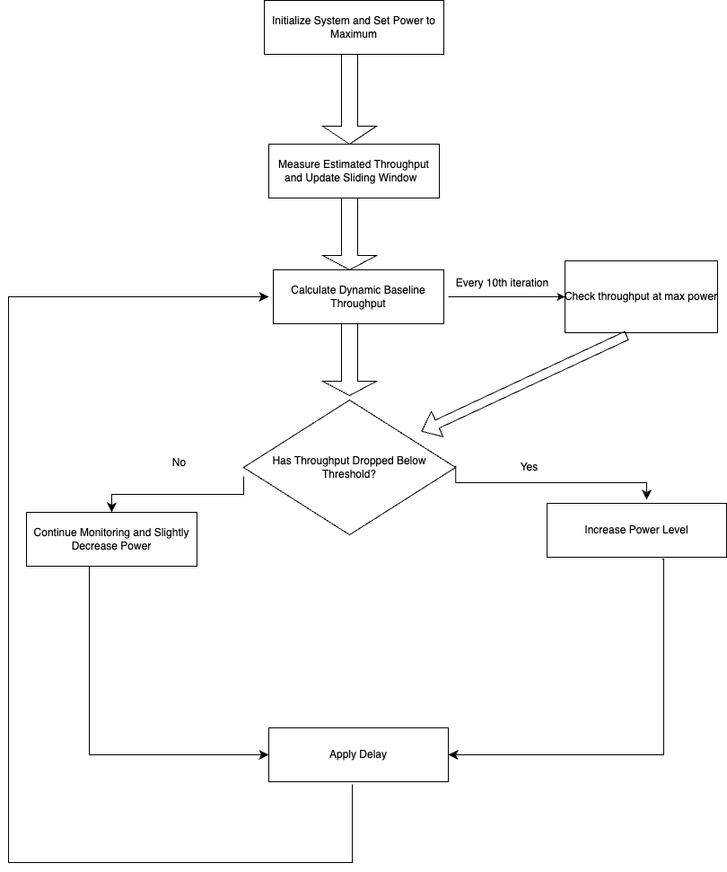
In this phase, we focused on refining the power control algorithm to dynamically adjust transmission power levels based on throughput measurements. Here’s a breakdown of the key steps and logic incorporated into the algorithm:
- Supported Power Levels: Each router or station has a list of supported power levels. This list is provided by the Python-WiFi-Manager, which serves as a critical component in our algorithm.
- Initial Assumption: We start with the assumption that the highest power level will yield the highest throughput. This serves as our baseline for evaluating other power settings.
- Algorithm Initialization: The algorithm begins by setting the transmission power to the highest level available. We then measure the expected throughput at this power level.
- Power Decrement: After measuring the expected throughput, we decrement the power level by one and take another measurement.
- Throughput Comparison: We assume a certain threshold that the throughputs at lower power can be below (for example 10% of) the previous throughput. If the expected throughput at the decreased power level falls below this threshold, we revert to the higher power level. This threshold ensures that the power is only decreased if the performance impact is minimal.
- Continued Decrease: If the throughput remains within an acceptable range, we continue to decrease the power level, repeating the measurement and comparison process.
- Iterative Process: This process is repeated iteratively, adjusting the power level based on throughput measurements until we reach the lowest supported power level.
- Periodic Maximum Power Check: Every 10th iteration, we re-evaluate the throughput at the maximum power level for a brief 60 ms. This ensures that the throughput at the current optimal power level, monitored for around 140 ms, remains within the threshold of the throughput measured at maximum power. Since we only stay at the maximum power for 60 ms, this approach minimizes the time spent at higher power levels, avoiding unnecessary power consumption.
- Adjust Based on Maximum Power Check: If the throughput at the optimal power level is still within the threshold of the maximum power throughput, we continue with our usual power adjustment process, either decreasing or maintaining the lowest power level.
- Fallback Strategy: If the throughput at the optimal power level falls below 90% of the throughput measured at the maximum power level (i.e., deviates by more than 10%), we restart the process using the second-highest power level to reassess and potentially find a better balance. All thresholds, including the deviation percentage and comparison intervals, are fully configurable.
This algorithm ensures a dynamic and adaptive approach to power control, optimizing network performance by continuously evaluating and adjusting based on real-time throughput data.
3. Determination of Expected Throughput
To effectively implement the power control algorithm, determining the expected throughput was crucial. Here’s how we enhanced the Python-WiFi-Manager to facilitate this:
- Extension of Python-WiFi-Manager: Extension of Python-WiFi-Manager: We extended the Python-WiFi-Manager package to include functionality for estimated throughput, which is derived from the Kernel Minstrel HT rate control algorithm. Minstrel HT maintains a rate table with expected throughput based on success probabilities for each transmission rate. The estimated throughput, obtained via Netlink, is calculated using the best rate (i.e., the expected throughput of the first rate in the MRR stage) determined by Minstrel HT. The reporting of estimated throughput from both the Python-WiFi-Manager package and Netlink is consistent and identical. By integrating this information, the Python-WiFi-Manager can now monitor and utilize these throughput estimates to optimize power control decisions in real-time.
- Extracting Optimal Rate: From the ‘best_rates’ lines provided by the Python-WiFi-Manager, we extracted the transmission rate that corresponds to the highest estimated throughput. This rate is a key indicator of potential performance at different power levels.
- Average Throughput Measurement: Using the optimal rate identified, we then referenced the ‘stats’ lines to extract the field for average throughput. This measurement represents the expected throughput at the given transmission rate and is essential for evaluating the effectiveness of different power settings.
- Integration into the Station Class: The extracted average throughput was integrated into the Station class of the Python-WiFi-Manager. We introduced a new property, ‘expected_throughput,’ to store this value. This property became a fundamental component of the power control algorithm, allowing real-time adjustments based on the estimated throughput.
By extending the Python-WiFi-Manager in this manner, we were able to leverage real-time throughput estimates effectively. This enhancement played a critical role in the development of our dynamic power control algorithm, enabling precise adjustments to optimize network performance.
4. Results from logging in the Power Controller
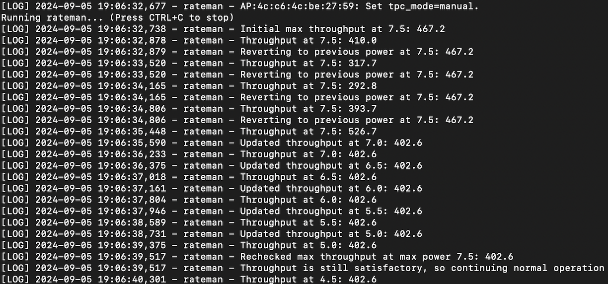
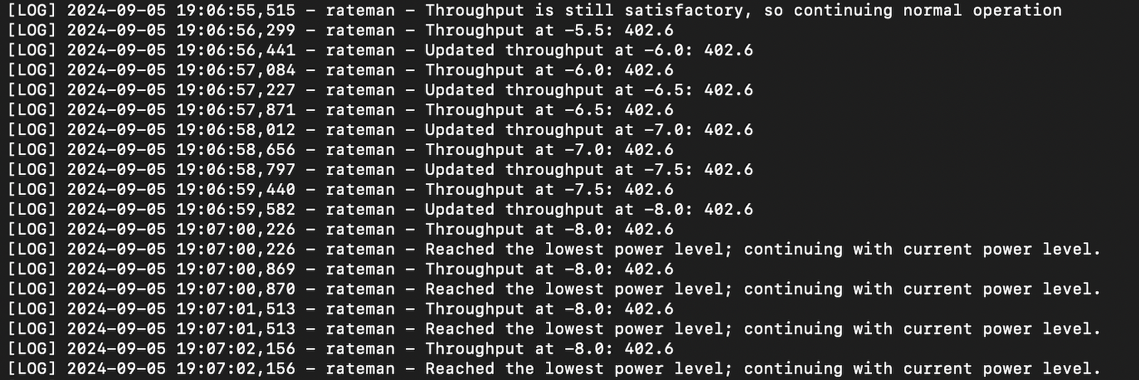
- Log Overview: The power controller logs capture a range of data points, including power levels, throughput measurements, and timestamps. These logs are crucial for understanding how the algorithm adjusts power settings in response to throughput changes.
- Key Data Points:
- Power Level Adjustments: Logs show each instance where the power level was adjusted, including the previous and new power levels.
- Throughput Measurements: Recorded throughput values at different power levels provide a basis for evaluating the effectiveness of power adjustments.
- Threshold Comparisons: Instances where the throughput fell below or met the predefined thresholds are noted, offering insight into the algorithm’s decision-making process.
3. Log Sample: Here’s a snapshot of the logs
5. Experimental Setup and Configuration
a. Access Point and Station Configuration
For the experiments, two Redmi Routers with MT768 chips were used, where one acted as the access point (AP) and the other as the station (STA). Both devices utilized IEEE 802.11ac(WiFi-5) capable.
- AP Configuration:
- The AP was configured to operate on the 5 GHz band using channel 149 with a maximum channel width of 80 MHz (VHT80).
- The 2.4 GHz band on the AP was disabled, focusing the experiment on the 5 GHz band for better throughput.
- STA Configuration:
- The STA was connected to the AP on the 5 GHz band, operating on the same channel (149).
- This setup ensured a controlled and consistent network environment for the experiments, particularly focusing on high-speed, 5 GHz communications between the devices.
b. Traffic Generation
Traffic was generated using iperf3, a tool widely used for network performance measurement. This allowed for the creation of a consistent and controlled load on the network, essential for evaluating the performance of the power control algorithm.
c. Throughput Calculation
Throughput was calculated using packet capture (pcap) files generated during the experiments. The process involved the following steps:
- Capture Data: During the experiments, network traffic was captured using tcpdump to generate pcap format to record detailed packet-level information.
- Convert to CSV: The pcap files were then converted into CSV format. This conversion facilitates easier analysis and manipulation of the data for calculating throughput.
- Data Analysis: The CSV files were analyzed to extract throughput metrics. This involved processing the data to determine the rate of successful data transmission between the Access Point (AP) and Station (STA).
This method allowed for precise measurement and post-experiment analysis of network performance.
d. Network Topology
In the close proximity experiments, the AP and STA were placed on the same table, approximately 2 meters apart, with no physical barriers between them. For the challenging conditions, the routers were positioned in different rooms or floors, with a distance of around 10 meters between them.
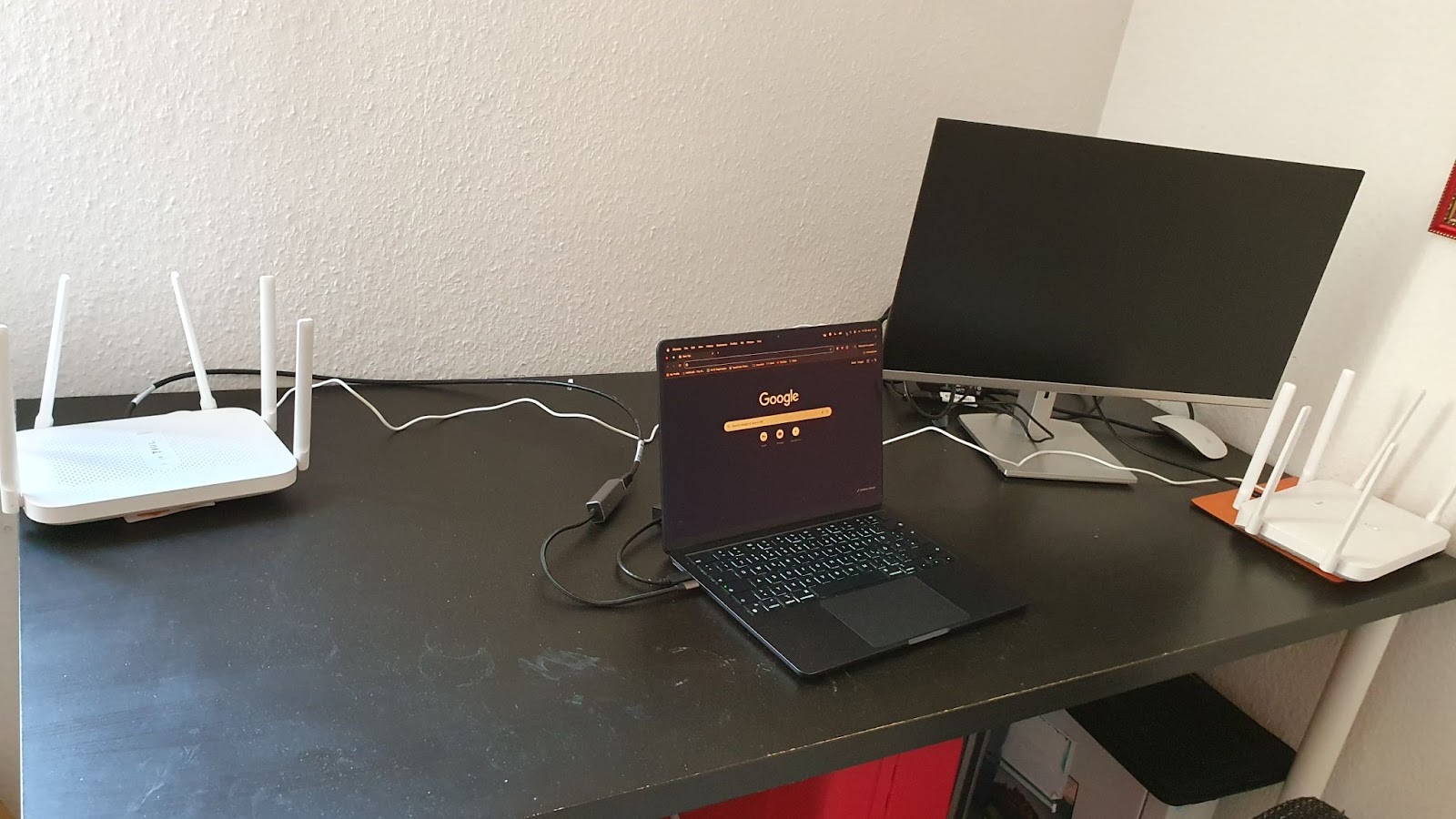
Fig. Experimental Setup in Close Proximity
6. Experimental Results
To evaluate the performance of our power control algorithm, the Experimentation Python package from SupraCoNex was utilized. This package facilitated a series of experiments conducted under various conditions to assess the algorithm’s effectiveness. Here’s a summary of the experimental approach and the results:
- Experimental Setup: Multiple experiments were conducted to test the power control algorithm in both close proximity and challenging conditions, allowing us to observe its performance across varied network environments.
- Data Extraction: From the experiments, we extracted key data related to rate-time, power-time, and throughput-time relationships. These data points are crucial for understanding how power adjustments impact throughput and rate over time.
- Data Visualization: The extracted data was then plotted to visualize the relationships:
- Rate vs. Time Plot: Shows how the transmission rate varies over time with different power levels.
- Power vs. Time Plot: Illustrates the power levels used during the experiments and how they change over time.
- Throughput vs. Time Plot: Displays the throughput variations over time, highlighting the performance of the algorithm in maintaining optimal throughput.
Analysis: By analyzing these plots, we were able to gain insights into how well the power control algorithm adapts to changing conditions and maintains network performance. The visualizations provided a clear picture of the algorithm’s effectiveness in real-time adjustments.
To evaluate the effectiveness of our power control algorithm, we compared it against several established methods. Here’s a brief overview of the algorithms used in the experiments:
1. Kernel Minstrel HT:
This algorithm focuses on selecting transmission rates based on observed performance metrics to optimize network performance. It employs a Multi-Rate Retry (MRR) strategy with four stages: the highest throughput rate (max_tp1), the second highest throughput rate(max_tp2), the third highest throughput rate (max_tp3), and the rate with the maximum success probability (max_prob_rate). If a rate at a given stage fails, the algorithm moves to the next stage in the sequence, ensuring continued performance optimization by using the next best available rate. This approach balances high throughput with reliable performance, adapting to varying network conditions.
2. Manual MRR Setter:
This method involves using a fixed, slower rate for all transmissions. By consistently using the slowest rate, this approach helps to understand the impact of rate adjustments and provides a reference point for evaluating dynamic control strategies. It provides a clear reference point for evaluating dynamic control strategies, helping to distinctly separate and identify the performance boundaries of different algorithms.
3. Our Power Controller:
Objective: The newly developed power control algorithm dynamically adjusts transmission power levels based on throughput measurements. It aims to optimize power settings to maintain high throughput while optimizing power and minimizing interference.
Mechanism: The algorithm starts with the highest power level, measures throughput, and progressively decreases power levels. It continuously checks throughput against predefined thresholds and adjusts power accordingly to maintain optimal performance.
A. Experiment in Close Proximity
With these algorithms set for comparison, the first set of experiments was conducted with the routers placed close to each other. The routers were positioned on the same table, approximately two meters apart with no barriers in between. This setup provided a controlled environment to accurately measure and compare the performance of each algorithm.
Observation: From the figure we can observe that if the connection is strong, the power controller can significantly reduce the power and still deliver high throughput.
B. Experiments under Challenging Conditions
Following the initial experiments with routers in close proximity, we conducted a second series of tests to evaluate the performance of the algorithms under more challenging conditions. For this phase, the routers were placed in different rooms and on different floors, approximately 10 meters apart. This setup was designed to simulate a more realistic scenario with increased distance, barriers and potential interference.
Observation:
Unlike the close-proximity experiments where power levels were dynamically adjusted, in the more distant setup, the power levels did not drastically reduce at all times. Instead, the natural tendency observed was for the power to stabilize at a lower level.
The power controller effectively managed to adjust the power levels, but the adjustments were more subtle compared to the previous tests. This is indicative of the controller’s ability to adapt to the increased distance and interference by settling at a lower, but stable, power level that still maintained acceptable throughput.
7. Possible Enhancements in the Future
While the current implementation of the power controller has demonstrated promising results, there are several immediate next steps to further enhance its performance and adaptability:
- Throughput Estimation Improvement: Study how well estimated throughput for optimal and highest power levels are isolated to provide better throughput estimates. This refinement could lead to more accurate power control decisions.
- Complex Scenario Testing: Test the controller in more complex scenarios involving other devices operating on the same channel. This will provide insights into how the controller performs in real-world conditions with multiple network elements.
- Interference Management: Conduct interference management tests with multiple access points (APs) and stations (STAs), all running the power controller. This will evaluate the system’s effectiveness in managing interference and maintaining performance in crowded environments.
In addition to these immediate enhancements, future developments could explore more advanced options such as leveraging machine learning for predictive adjustments, utilizing historical data for better adaptability, implementing time-of-day adjustments for optimized power settings, and adapting to environmental factors for improved robustness.
Conclusion
I’ve had an incredible experience being part of GSoC 2024. This opportunity has allowed me to delve into new areas, including working with Python for the first time and developing plotting scripts. I am truly grateful for the chance to contribute to this project and learn so much along the way. A big thank you to the mentors who provided invaluable support and guidance throughout the journey.